Epsilon-Delta & Continuity
From sequence limits to function limits — the ε-δ definition, continuity, the Intermediate and Extreme Value Theorems, and the Lipschitz condition that controls gradient descent
Abstract. A function f has limit L at a if for every ε > 0, there exists δ > 0 such that 0 < |x - a| < δ implies |f(x) - L| < ε. This ε-δ definition extends the ε-N framework for sequences to arbitrary functions and serves as the foundation for all subsequent calculus. Continuity at a point means the limit equals the function value — equivalently, small perturbations in the input produce small perturbations in the output. The Intermediate Value Theorem guarantees that continuous functions on intervals cannot 'skip' values, which implies the existence of roots and decision boundaries. The Extreme Value Theorem guarantees that continuous functions on closed, bounded intervals attain their maximum and minimum — the theoretical foundation for the existence of optimal parameters in constrained optimization. Beyond pointwise continuity, Lipschitz continuity — |f(x) - f(y)| ≤ K|x - y| — quantifies how 'well-behaved' a function is. In machine learning, the Lipschitz constant of the loss gradient directly controls gradient descent convergence rates, spectral normalization enforces Lipschitz constraints on neural network layers for Wasserstein GANs, and the continuity properties of activation functions (ReLU is continuous but not differentiable; sigmoid is smooth with K = 1/4) determine whether gradient-based training is possible at all.
Overview & Motivation
Picture a loss function landscape — a surface where each point represents a set of model parameters and its height represents the loss. When we nudge the parameters slightly, does the loss change by a small, predictable amount? Or could it jump discontinuously, making gradient-based optimization impossible? If we know one set of parameters gives positive loss and another gives negative loss, must there be parameters that give exactly zero loss?
These are questions about continuity, and the ε-δ framework we develop here makes them precise. Continuity is the minimal requirement for gradient-based optimization: if the loss function is not continuous, we cannot even define a meaningful gradient, let alone follow it downhill.
In Sequences, Limits & Convergence, we made “arbitrarily close” precise for sequences with the ε-N definition: for all . Now we extend this framework to functions. Instead of asking “what happens as gets large?”, we ask “what happens as approaches a point ?” The machinery is analogous — we still quantify “for every ε, there exists…” — but the ε-δ definition for functions is subtler because δ can depend on both ε and the point .
The ε-δ Definition of a Function Limit
From intuition to precision
We want to say ” approaches as approaches .” Informally, this means: as we take values closer and closer to , the corresponding values get closer and closer to .
Our first attempt at making this precise: “for close to , is close to .” But how close is “close”? We need to quantify both closeness conditions — and the key insight is that the first one (how close is to ) should be a response to the second one (how close we want to be to ).
This gives us the quantifier structure: for every closeness requirement on , there exists a sufficient closeness requirement on .
📐 Definition 1 (Limit of a Function)
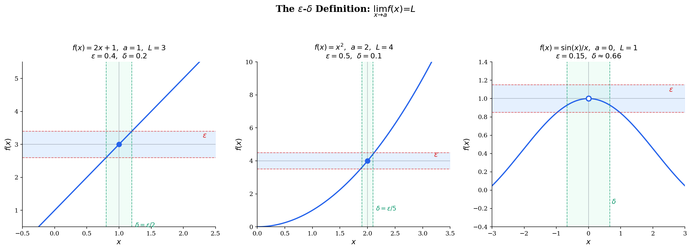
Let be defined on an open interval containing , except possibly at itself. We say if for every , there exists such that
We write as .
The condition is critical: we require . The limit describes the behavior of near , not at . The function need not even be defined at — all that matters is what happens in every punctured neighborhood of .
Geometrically, the ε-δ definition says: draw a horizontal band of width centered at . No matter how narrow this band, we can find a vertical band of width centered at such that the function graph inside the vertical band stays inside the horizontal band. The intersection of these bands forms an “ε-δ box,” and the function graph must stay inside the box.
Worked examples
📝 Example 1 (Proof that lim(2x + 1) = 3 as x → 1)
Claim: .
Proof. Let be given. We need to find such that implies .
We work backward from the conclusion:
So is equivalent to , which is .
Choose . Then implies
For linear functions, the algebra is clean: is simply divided by the slope. But for nonlinear functions, we need to be more careful.
📝 Example 2 (Proof that lim x² = 4 as x → 2)
Claim: .
Proof. Let be given. We need such that implies .
Factor: . The challenge is that depends on , so we need to bound it. If we restrict , then means , so .
Under this restriction: .
Choose . Then implies:
- , so
- , so
Therefore .
The “restrict δ first to bound a factor, then choose δ as a minimum” technique is the standard approach for polynomial and rational limits. The key step — bounding by restricting to a neighborhood of — is where the real work happens.
A non-example: Consider at . As , the function oscillates between and infinitely often. For any candidate limit and any , no matter how small we make , the interval contains points where and points where . No single can be within of both. Therefore does not exist.
🔷 Proposition 1 (Uniqueness of Limits)
If exists, it is unique. That is, if and , then .
Proof.
Suppose and with . Set . By the limit definition, there exist such that:
Let and pick any with . By the triangle inequality:
This gives , a contradiction. Therefore .
Try dragging the ε slider below to see the ε-δ box shrink around the limit. As ε decreases, δ must decrease too — the box tightens, but the function graph always stays inside it.
One-Sided Limits and Limits at Infinity
Sometimes we care about the behavior of as approaches from only one side. This is essential for functions with different behavior on the left and right — like the floor function at integers, or ReLU at 0.
📐 Definition 2 (Left-Hand Limit)
We say if for every , there exists such that
📐 Definition 3 (Right-Hand Limit)
We say if for every , there exists such that
🔷 Proposition 2 (Two-Sided Limit from One-Sided Limits)
if and only if and .
Proof.
Forward direction. If , then for every there exists such that implies . This condition includes both and , so both one-sided limits equal .
Reverse direction. Suppose both one-sided limits equal . Given , there exist such that:
Set . Then means either or , and in either case .
📐 Definition 4 (Limit at Infinity)
We say if for every , there exists such that
Similarly, if for every , there exists such that implies .
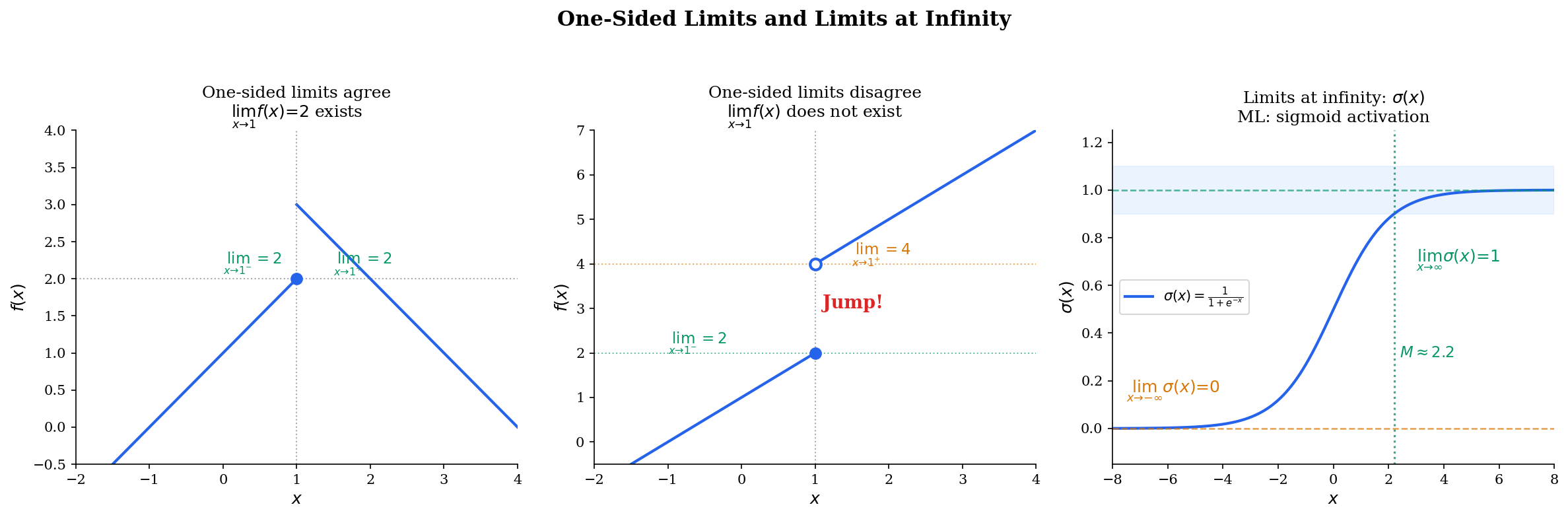
ML context: One-sided limits appear at ReLU’s kink at 0. The left-hand limit of as is 0, and the right-hand limit as is 1. Since both one-sided limits of the function itself exist and equal 0, ReLU is continuous at 0 — even though it is not differentiable there. Limits at infinity describe the asymptotic behavior of sigmoid ( as ) and tanh ( as ).
Continuity at a Point
A function is continuous at a point if there is no “break” in its graph there. The formal definition captures three conditions that must all hold.
📐 Definition 5 (Continuity at a Point)
A function is continuous at if:
- is defined,
- exists, and
- .
Equivalently: for every , there exists such that implies .
We say is continuous on an interval if is continuous at every point of .
Notice the subtle difference from the limit definition: we write (not ). For continuity, we include itself — and condition 3 ensures that is the “right” value.
The sequential characterization provides a powerful bridge back to Topic 1.
🔷 Theorem 1 (Sequential Characterization of Continuity)
A function is continuous at if and only if for every sequence with , we have .
Proof.
Forward direction. Assume is continuous at , and let be a sequence with . Given , by continuity there exists such that implies . Since , there exists such that implies . For such , we have . This proves .
Reverse direction (contrapositive). Assume is not continuous at . Then there exists such that for every , there is some with but . For each , apply this with : there exists with but . Then (since ) but (since for all ).
💡 Remark 1 (Bridge Between Topics 1 and 2)
The sequential characterization is the bridge between sequence convergence (Topic 1) and function continuity (this topic). It lets us apply all the sequence-convergence theorems — Monotone Convergence, Squeeze, Bolzano-Weierstrass, the Algebra of Limits — in the function setting. When we need to prove something about a continuous function, we can often reduce it to a statement about convergent sequences, where we already have powerful tools.
Algebra of Continuous Functions
🔷 Theorem 2 (Algebra of Continuous Functions)
If and are continuous at , then so are:
- and
- (provided )
- (if is continuous at and is continuous at )
Proof.
We prove this via the sequential characterization. Let be any sequence with . Since and are continuous at , we have and .
Sum: By the Algebra of Limits for sequences (Theorem 3 from Sequences, Limits & Convergence), .
Product: Similarly, .
Quotient: If , then by the quotient rule for sequences.
Composition: If is continuous at , then . If is continuous at , then . This shows .
🔷 Corollary 1 (Continuity of Polynomials and Rational Functions)
Every polynomial is continuous on . Every rational function is continuous on its domain (wherever ).
💡 Remark 2 (Continuity of Neural Networks)
In machine learning, this theorem is why compositions of continuous layers produce continuous networks. If each activation function is continuous and each affine map is continuous (which it is, as a polynomial), then the full network
is continuous by iterated application of the composition rule. This is the minimal requirement for the network to have well-defined gradients almost everywhere.
Types of Discontinuities
Not all discontinuities are created equal. Understanding the classification tells us what can be “fixed” and what cannot.
📐 Definition 6 (Removable Discontinuity)
A function has a removable discontinuity at if exists, but either is undefined or . Redefining “removes” the discontinuity.
📐 Definition 7 (Jump Discontinuity)
A function has a jump discontinuity at if both one-sided limits and exist, but .
📐 Definition 8 (Essential Discontinuity)
A function has an essential discontinuity at if at least one of the one-sided limits fails to exist (either diverges to infinity or oscillates).
Concrete examples:
- Removable: at — the limit is 1, but the function is undefined at 0.
- Jump: (floor function) at any integer — left and right limits differ by 1.
- Essential: at — infinite oscillation, no limit exists.
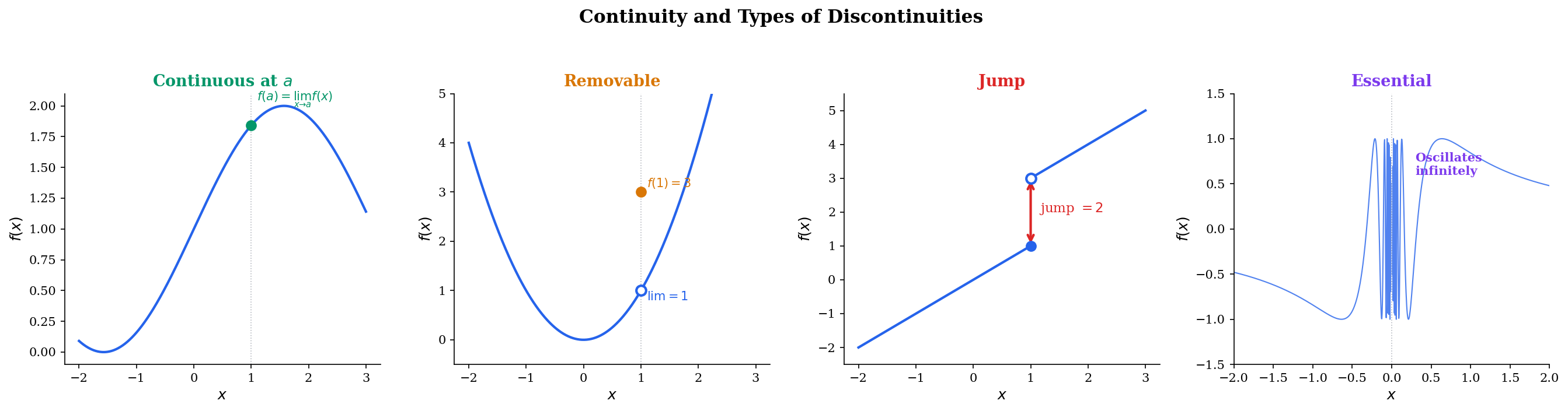
Explore the four types below. The ε-δ box shows why continuity fails for each type: for the continuous case, a valid δ always exists. For removable discontinuities, the limit exists but misses f(a). For jump discontinuities, no single δ-band can contain both sides. For essential discontinuities, the oscillation defeats any ε.
The Intermediate Value Theorem
The IVT is one of the most intuitive theorems in analysis — a continuous function cannot “jump” over a value — but its proof requires the completeness of .
🔷 Theorem 3 (Intermediate Value Theorem)
Let be continuous. If is any value between and , then there exists such that .
Proof.
Without loss of generality, assume (the case follows by applying the argument to ).
Define . This set is non-empty (it contains , since ) and bounded above by . By the completeness of (the least upper bound property), exists.
We claim . We rule out the other two possibilities:
Case 1: . Set . By continuity, there exists such that implies , i.e., . Since (because ), the interval for is non-empty, and every in this interval satisfies , hence . But then is not an upper bound of — contradiction with .
Case 2: . Set . By continuity, there exists such that implies . So no point in belongs to . But means every interval must contain points of — contradiction.
Both cases lead to contradictions, so .
🔷 Corollary 2 (Root Existence)
If is continuous on and (i.e., changes sign), then there exists with .
💡 Remark 3 (IVT and Decision Boundaries)
The IVT is the theoretical foundation of the bisection method for root-finding. More broadly, it guarantees the existence of decision boundaries: if a continuous classifier assigns a positive score to one data point and a negative score to another, the IVT guarantees that somewhere between them, the classifier outputs exactly zero — a decision boundary exists. This is why continuous classifiers always produce connected decision regions.
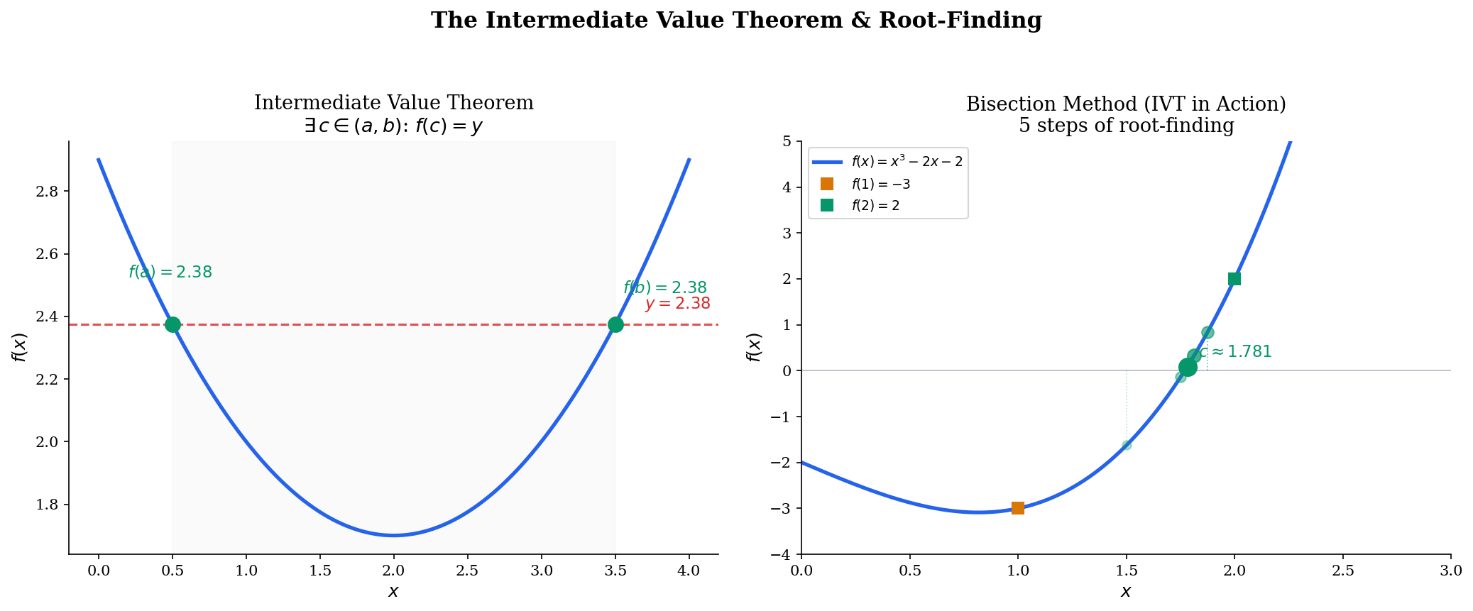
Drag the horizontal target line to see IVT in action. Toggle bisection mode to watch the algorithm narrow in on the root step by step.
The Extreme Value Theorem
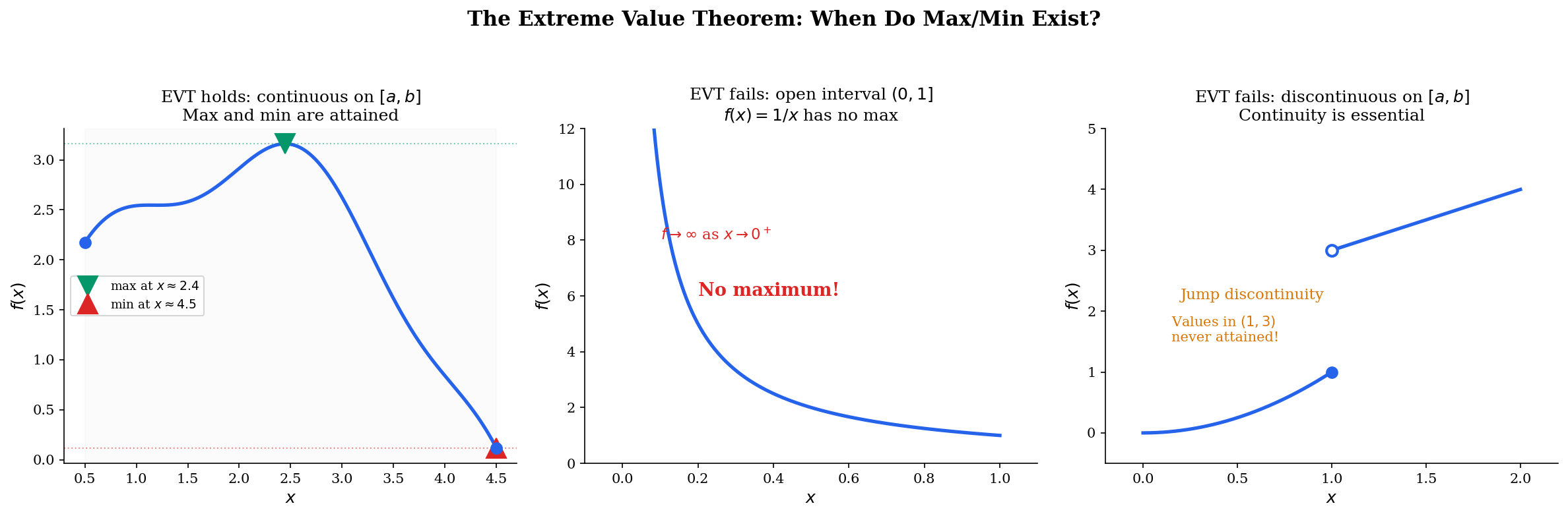
🔷 Theorem 4 (Extreme Value Theorem)
If is continuous, then attains its maximum and minimum on . That is, there exist such that for all .
Proof.
We prove the maximum case; the minimum case follows by applying the argument to .
Step 1: is bounded above on . Suppose not. Then for each , there exists with . The sequence is bounded (all terms lie in ), so by the Bolzano-Weierstrass Theorem (from Sequences, Limits & Convergence), there is a convergent subsequence (the interval is closed, so the limit stays in ). By continuity, . But , which contradicts convergence. Therefore is bounded above.
Step 2: The supremum is attained. Let , which exists by Step 1. By the definition of supremum, for each there exists with . Again by Bolzano-Weierstrass, extract a convergent subsequence . By continuity, . Since for all , we get by the Squeeze Theorem.
💡 Remark 4 (EVT and Optimization)
The EVT is the existence theorem for optimization: it guarantees that has a solution when is continuous and the domain is compact (closed and bounded). In machine learning, regularization and weight clipping create compact parameter spaces — for example, constraining — precisely to ensure that minimizers exist. Without compactness, a continuous function may approach but never reach its infimum (think of on , which approaches 0 but never reaches it).
Uniform Continuity and Lipschitz Continuity
So far, our notion of continuity is pointwise: at each point , we find a δ that works for that specific . But δ might shrink as moves — different points might need different δ values. Uniform continuity asks for a single δ that works everywhere simultaneously.
📐 Definition 9 (Uniform Continuity)
A function is uniformly continuous on a set if for every , there exists such that for all :
The key difference: in pointwise continuity, depends on both and the point . In uniform continuity, depends only on — the same δ works for every pair of points in .
Lipschitz continuity goes further: it demands a linear relationship between input perturbation and output perturbation.
📐 Definition 10 (Lipschitz Continuity)
A function is Lipschitz continuous with constant on a set if
The smallest such is called the Lipschitz constant of on .
Geometrically, is -Lipschitz if and only if at every point , the graph of stays inside a cone with slopes . The Lipschitz constant is the steepest the function is allowed to be — anywhere.
🔷 Proposition 3 (The Continuity Hierarchy)
Lipschitz continuity uniform continuity (pointwise) continuity.
Both converses are false.
Proof.
Lipschitz uniform continuity. Given , choose . Then implies . This depends only on (not on or ), so is uniformly continuous.
Uniform continuity continuity. Immediate: uniform continuity at every pair with near gives pointwise continuity at .
Counterexample for first converse: on is uniformly continuous (continuous on a compact set — Heine-Cantor, Theorem 5 below) but not Lipschitz: as .
Counterexample for second converse: on is continuous but not uniformly continuous. For any , take and . Then but . So has no valid .
🔷 Theorem 5 (Heine-Cantor Theorem)
If is continuous on a compact set (closed and bounded in ), then is uniformly continuous on .
💡 Remark 5 (Compactness Upgrades Continuity)
The Heine-Cantor theorem explains why compactness is so important for optimization. On compact domains, continuity automatically gives us uniform continuity — uniform control over function behavior everywhere. This is the machinery behind many existence and approximation theorems in analysis and ML, and we develop it fully in Completeness & Compactness.
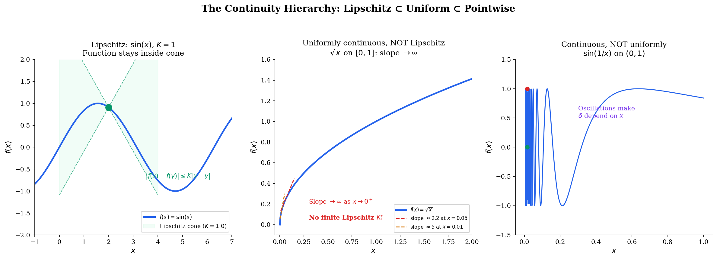
Drag the point along the function to see the Lipschitz cone follow. Adjust to see how the constraint tightens. For , notice how the cone fails near — the slope blows up, so no finite works.
Connections to Statistics
The ε-δ definition of continuity is what makes the Continuous Mapping Theorem and the functional delta method work — small probabilistic technicalities that turn out to be load-bearing.
Convergence in distribution and continuity points
Convergence in distribution requires pointwise convergence at every continuity point of . The ε-δ definition is precisely what this qualifier means. The Continuous Mapping Theorem — if in probability and is continuous at , then — directly composes ε-δ continuity with probabilistic convergence. See formalStatistics Modes of Convergence.
The functional delta method
The functional delta method and continuous mapping arguments in empirical-process theory are ε-δ statements lifted to Banach-valued random elements. Continuity of functionals in the sup-norm metric is the key hypothesis that makes the delta method extend from real-valued to function-valued estimators. See formalStatistics Empirical Processes.
Connections to ML
Activation function continuity
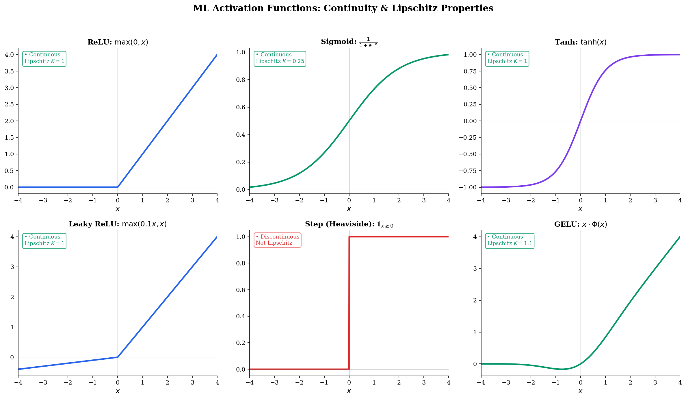
The continuity properties of activation functions determine whether gradient-based training is possible at all.
- ReLU : Continuous everywhere (both one-sided limits agree at 0). Lipschitz with . Not differentiable at 0, but the subgradient exists.
- Sigmoid : Smooth (infinitely differentiable). Lipschitz with (maximum slope at ).
- Tanh : Smooth. Lipschitz with .
- GELU : Smooth. Lipschitz with .
- Step function : Discontinuous at 0 (jump). Cannot be trained with gradient descent — gradients are zero almost everywhere.
The step function illustrates why continuity matters: its discontinuity makes gradient-based optimization impossible, which is why smooth approximations (sigmoid, softmax) replaced it in neural network training. See formalML Gradient Descent for the full convergence analysis.
Loss landscape smoothness
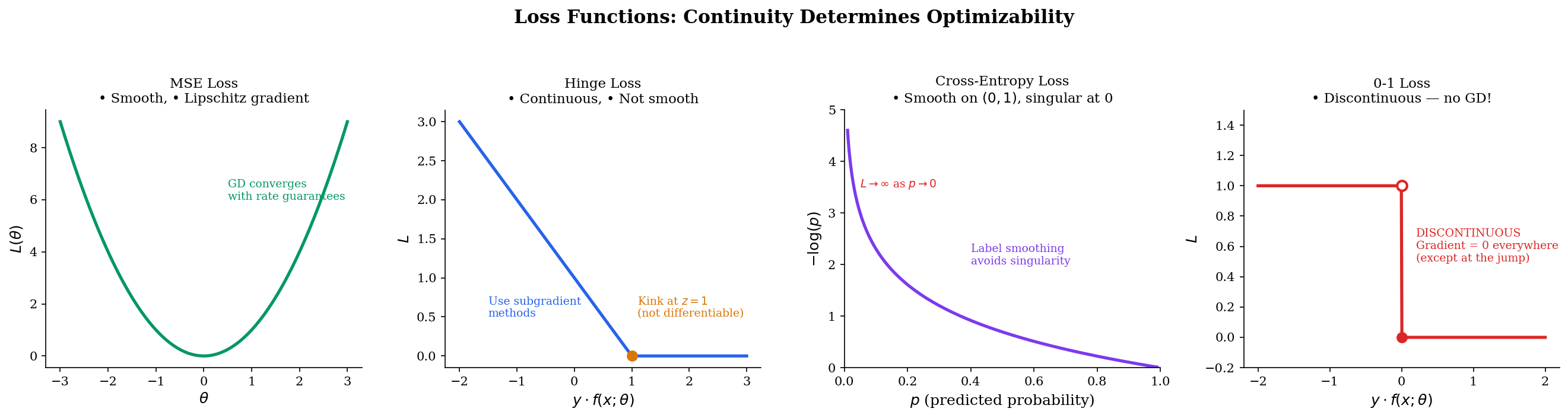
Different loss functions have different continuity properties, which determines which optimization methods apply:
- MSE : Smooth, Lipschitz gradient. Gradient descent converges.
- Hinge : Continuous but not differentiable at . Subgradient methods work.
- Cross-entropy : Smooth on but singular at (loss ). Requires clipping or label smoothing.
- 0-1 loss : Discontinuous. Not trainable with gradients — this is why we use continuous surrogates.
See formalML Convex Analysis for the full treatment of loss function properties.
Lipschitz constraints in GANs
The Wasserstein GAN (WGAN) critic must be 1-Lipschitz to ensure the Wasserstein distance is well-defined (Kantorovich-Rubinstein duality). The original paper enforced this via weight clipping: . Spectral normalization (Miyato et al., 2018) provides a tighter enforcement by normalizing each weight matrix by its spectral norm :
This ensures the Lipschitz constant of the network is at most 1, since the Lipschitz constant of a composition is bounded by the product of the layer-wise constants. The trade-off: smaller means a more constrained (less expressive) critic, but more stable training.
IVT and decision boundaries
If a continuous classifier assigns a positive score to one data point and a negative score to another, the IVT guarantees that along any continuous path between them, there exists a point where — a decision boundary. This means continuous classifiers always produce well-defined, connected decision regions. Discontinuous classifiers can create “islands” with no clear boundary. See formalML PAC Learning for how continuity assumptions on hypothesis classes affect learnability.
Computational Notes
Evaluating limits numerically
import numpy as np

def numerical_limit(f, a, n_steps=20):
    """Evaluate lim_{x->a} f(x) by approaching from both sides."""
    h_values = [10**(-k * 0.5) for k in range(1, n_steps + 1)]
    left = [f(a - h) for h in h_values]
    right = [f(a + h) for h in h_values]
    print(f"Left:  {left[-1]:.12f}")
    print(f"Right: {right[-1]:.12f}")
    return (left[-1] + right[-1]) / 2

# Example: lim_{x->0} sin(x)/x = 1
numerical_limit(lambda x: np.sin(x) / x, 0)
Estimating Lipschitz constants
def estimate_lipschitz(f, a, b, n=10000):
    """Estimate the Lipschitz constant of f on [a, b]."""
    x = np.linspace(a, b, n)
    fx = f(x)
    max_ratio = 0
    for i in range(n - 1):
        ratio = abs(fx[i+1] - fx[i]) / abs(x[i+1] - x[i])
        max_ratio = max(max_ratio, ratio)
    return max_ratio

# sin(x) on [-pi, pi]: K should be close to 1
K = estimate_lipschitz(np.sin, -np.pi, np.pi)
print(f"Lipschitz constant of sin(x): {K:.4f}")
Bisection root-finding
def bisection(f, a, b, tol=1e-10, max_iter=100):
    """Find root of f in [a, b] using the bisection method (IVT)."""
    assert f(a) * f(b) < 0, "f must change sign on [a, b]"
    for i in range(max_iter):
        mid = (a + b) / 2
        if abs(f(mid)) < tol or (b - a) / 2 < tol:
            return mid, i + 1
        if f(a) * f(mid) < 0:
            b = mid
        else:
            a = mid
    return (a + b) / 2, max_iter

# Find root of x^3 - 2x - 2 in [0, 3]
root, iters = bisection(lambda x: x**3 - 2*x - 2, 0, 3)
print(f"Root: {root:.10f} (found in {iters} iterations)")
Connections & Further Reading
Where this leads — next in formalCalculus
On to formalStatistics — where this calculus powers inference
Modes Of Convergence
Convergence in distribution F_n ⟹ F requires pointwise convergence at every continuity point of F. The ε-δ definition of continuity is what this 'continuity point' qualifier means. The Continuous Mapping Theorem directly composes ε-δ continuity with probabilistic convergence.
Empirical Processes
The functional delta method and continuous mapping arguments in empirical-process theory are ε-δ statements lifted to Banach-valued random elements. Continuity of functionals T: D[0,1] → ℝ in the sup-norm metric is the key hypothesis.
On to formalML — where this calculus powers ML
Convex Analysis
Convex functions on open sets are automatically continuous — a non-trivial theorem. Semicontinuity generalizes continuity for optimization, and the Lipschitz gradient condition (∇f is L-Lipschitz) is the key assumption in gradient descent convergence proofs.
Gradient Descent
The convergence rate of gradient descent on smooth functions depends on the Lipschitz constant of the gradient: step size η must satisfy η < 2/L for L-smooth functions. The continuity of the loss landscape is the minimal requirement for gradient-based optimization.
PAC Learning
Continuous hypothesis classes and the uniform convergence of empirical risk to true risk rely on continuity and compactness arguments developed here.
References
- book Abbott (2015). Understanding Analysis Chapter 4 develops continuity with the ε-δ definition and proves IVT and EVT — the primary reference for our exposition
- book Rudin (1976). Principles of Mathematical Analysis Chapter 4 on continuity — the definitive compact treatment of uniform continuity and compactness
- book Tao (2016). Analysis I Chapter 9 on continuous functions and Chapter 13 on uniform continuity — first-principles construction with careful scaffolding
- book Boyd & Vandenberghe (2004). Convex Optimization Section 2.2 on convex function continuity, Section 9.3 on Lipschitz gradient conditions for convergence
- paper Arjovsky, Chintala & Bottou (2017). “Wasserstein Generative Adversarial Networks” The 1-Lipschitz constraint on the WGAN critic is a direct application of Lipschitz continuity to generative modeling
- paper Miyato, Kataoka, Koyama & Yoshida (2018). “Spectral Normalization for Generative Adversarial Networks” Spectral normalization enforces the Lipschitz constraint by normalizing weight matrices by their spectral norm