The Riemann Integral & FTC
Area as a limit of sums — the Riemann integral defined via partitions and Darboux sums, integrability of continuous functions, and the Fundamental Theorem connecting differentiation and integration
Abstract. The Riemann integral formalizes the intuitive notion of 'area under a curve' as a limit of finite sums. Given a function f on [a,b] and a partition P = {x₀, x₁, ..., xₙ} of [a,b], a Riemann sum Σ f(tᵢ) Δxᵢ approximates the integral by summing the areas of narrow rectangles. The integral ∫ₐᵇ f(x) dx is the common value of the upper and lower Darboux sums — sup Σ Mᵢ Δxᵢ and inf Σ mᵢ Δxᵢ — when they agree in the limit of partition refinement. Continuous functions on [a,b] are always Riemann integrable: uniform continuity (guaranteed by compactness of [a,b]) ensures that the upper and lower sums can be made arbitrarily close by choosing a fine enough partition. The Fundamental Theorem of Calculus forges the link between differentiation and integration. Part 1 says that if f is continuous, the area function F(x) = ∫ₐˣ f(t) dt is differentiable with F'(x) = f(x) — integration followed by differentiation recovers the original function. Part 2 says that if F is any antiderivative of f, then ∫ₐᵇ f(x) dx = F(b) - F(a) — the integral is computed by evaluating the antiderivative at the endpoints. The proof of Part 2 uses the Mean Value Theorem to relate the telescoping sum F(b) - F(a) = Σ [F(xᵢ) - F(xᵢ₋₁)] to the Riemann sum Σ f(cᵢ) Δxᵢ. Substitution (u-substitution) is the chain rule in reverse: ∫ f(g(x))g'(x) dx = ∫ f(u) du. Integration by parts is the product rule in reverse: ∫ u dv = uv - ∫ v du. In machine learning, the integral is ubiquitous: expected values E[X] = ∫ x f(x) dx, loss functions as integrals over distributions, marginalizing over latent variables, and probability computations all require integration. Numerical quadrature — trapezoidal rule, Simpson's rule, Gaussian quadrature — provides the computational tools when antiderivatives don't exist in closed form.
Overview & Motivation
You’re computing the expected loss of a model over a continuous data distribution: . What does this integral mean, precisely? It’s the limit of a sum: partition the input space into small regions, compute the loss density volume in each region, and sum up. As the regions shrink, the sum converges to the integral. This is not a metaphor — it’s the definition.
The Riemann integral makes “area under a curve” (and its higher-dimensional generalizations) rigorous. We’ll define it via partitions and Darboux sums (§2–3), prove that continuous functions are integrable (§4), establish the Fundamental Theorem of Calculus that ties integration to differentiation (§6–7), develop the key integration techniques (§8), and connect everything to expected values and numerical computation in ML (§11).
Prerequisites: We use the sequence convergence framework from Sequences, Limits & Convergence, the epsilon-delta characterization of uniform continuity from Epsilon-Delta & Continuity, the Heine-Cantor theorem from Completeness & Compactness, and the Mean Value Theorem from Mean Value Theorem & Taylor Expansion.
Partitions and Riemann Sums
The geometric picture
Start with a curve above the -axis on . Slice the interval into equal subintervals. In each subinterval, build a rectangle whose height is the function value at some sample point. The total area of these rectangles approximates the area under the curve. The approximation improves as the slices get thinner — and the Riemann integral is the limit of this process.
📐 Definition 1 (Partition)
A partition of is a finite ordered set with . The mesh (or norm) of is where . A partition is a refinement of if (every point of is also a point of ).
📐 Definition 2 (Riemann Sum)
Given a bounded function , a partition , and sample points for each , the Riemann sum is
Specific choices of sample points yield named rules:
- Left rule: (left endpoint of each subinterval)
- Right rule: (right endpoint)
- Midpoint rule: (midpoint)
📝 Example 1 (Riemann sums for f(x) = x² on [0, 1])
Take the uniform partition with subintervals, so and the partition points are .
Left sum:
Right sum:
The exact integral is , which is trapped between the left and right sums (as expected for this increasing function). As grows, both sums converge to .
💡 Remark 1 (The trapezoidal rule)
Average the left and right Riemann sums to get the trapezoidal rule:
Geometrically, each rectangle is replaced by a trapezoid whose top edge connects to . This typically gives a better approximation than either endpoint rule alone, because the trapezoid’s area is the average of the over-estimate and under-estimate.
![Three-panel illustration: left, right, and midpoint Riemann sums for x² on [0,1] with n = 8](/images/topics/riemann-integral/riemann-sums.png)
Upper and Lower Sums — The Darboux Approach
Why Darboux?
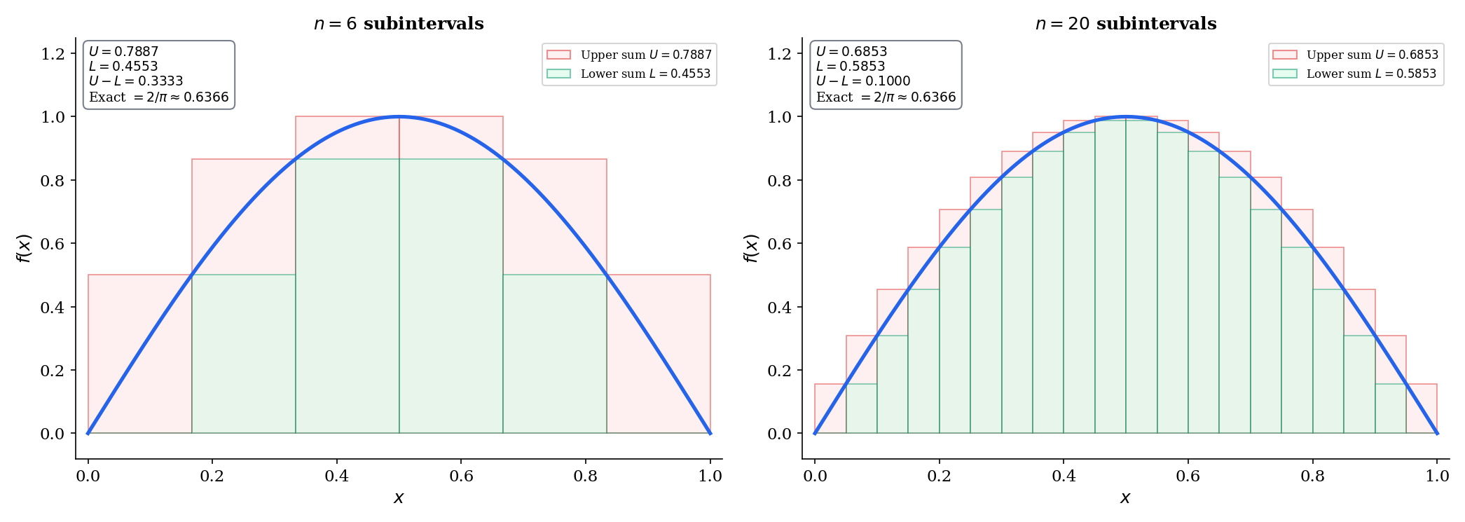
Riemann sums depend on the choice of sample points . To define the integral without this ambiguity, we bound the sums from above and below using suprema and infima of on each subinterval. This is the Darboux approach, and it gives us a clean criterion for integrability: the integral exists if and only if the upper and lower bounds can be squeezed arbitrarily close.
📐 Definition 3 (Upper and Lower Darboux Sums)
For a bounded function on and a partition , define
The upper Darboux sum is and the lower Darboux sum is .
For any choice of sample points, .
🔷 Proposition 1 (Refinement Monotonicity)
If is a refinement of , then
Refining a partition increases lower sums and decreases upper sums — the bounds get tighter.
Proof.
It suffices to show the result when is obtained by adding a single point to , since the general case follows by induction on the number of added points.
On the subinterval , the upper sum contributes where . Splitting at gives two subintervals and with suprema
So the new contribution is
All other subintervals are unchanged, so . The argument for is analogous (infima on smaller subintervals are the infimum on the larger subinterval).
🔷 Proposition 2 (Upper-Lower Inequality)
For any partitions and (not necessarily related by refinement), .
Proof.
The common refinement refines both and . By Proposition 1:
The middle inequality holds because on every subinterval.
The Riemann Integral
📐 Definition 4 (The Riemann Integral (Darboux Definition))
A bounded function is Riemann integrable if the upper and lower integrals agree:
The common value is written and called the Riemann integral of on .
💡 Remark 2 (Equivalent ε-characterization of integrability)
is Riemann integrable if and only if for every , there exists a partition such that . This is the criterion we’ll use in all integrability proofs: show that the gap between upper and lower sums can be made as small as we like.
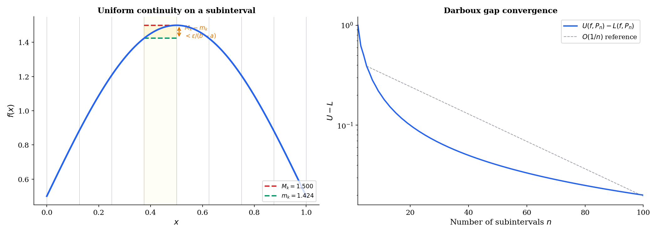
🔷 Theorem 1 (Continuous Functions Are Riemann Integrable)
If is continuous, then is Riemann integrable.
Proof.
Since is compact (Heine-Borel, Completeness & Compactness), is uniformly continuous on (Heine-Cantor theorem, also from Topic 3).
Given , choose such that
Take any partition with mesh . On each subinterval , the length is , so for any we have . In particular:
Therefore:
Every step is explicit. The chain compactness uniform continuity integrability is fully traced.
🔷 Theorem 2 (Monotone Functions Are Riemann Integrable)
If is monotone (either increasing or decreasing throughout), then is Riemann integrable.
Proof.
Assume is increasing (the decreasing case is analogous). For any partition , the supremum on is and the infimum is — since is increasing.
With the uniform partition :
The sum telescopes: .
So . Given , choose .
📝 Example 2 (The Dirichlet function is not Riemann integrable)
Define if and if . On any subinterval :
- because the rationals are dense — every subinterval contains rational numbers.
- because the irrationals are dense — every subinterval contains irrational numbers.
So and for every partition . The upper and lower integrals disagree: , so is not Riemann integrable.
This example matters for ML: the Dirichlet function is a legitimate measurable function, and the Lebesgue integral can handle it (). The failure of Riemann integration for such functions is precisely why measure-theoretic probability (→ formalML: Measure-Theoretic Probability) requires the more powerful Lebesgue integral.
💡 Remark 3 (Bounded functions with finitely many discontinuities)
If is bounded on and has only finitely many points of discontinuity, then is still Riemann integrable. The idea: cover the discontinuities with subintervals of arbitrarily small total length (contributing at most to ), and handle the continuous portions with Theorem 1. Discontinuities on a set of “measure zero” don’t spoil integrability — a fact that foreshadows the Lebesgue criterion.
Properties of the Integral
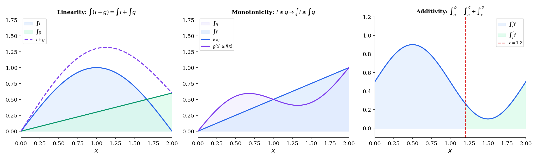
🔷 Theorem 3 (Properties of the Riemann Integral)
If and are Riemann integrable on and :
(a) Linearity:
(b) Monotonicity: If for all , then .
(c) Additivity over intervals: For any :
(d) Triangle inequality:
Proof.
(a) Linearity (additivity). For any partition , the infimum of a sum satisfies on each subinterval. Therefore . Similarly, . Taking the supremum of lower sums and infimum of upper sums gives
So all four quantities are equal. The scalar multiplication follows by similar reasoning (with separate cases for and ).
(b) Monotonicity. If on , then for every partition (the infimum of on each subinterval is the infimum of ). Taking gives .
(c) Additivity. Use a common refinement that includes the point . On such a refinement, the Riemann sums over split exactly into sums over and .
(d) Triangle inequality. Since for all , apply monotonicity: , which gives .
📝 Example 3 (Computing ∫₀¹ x² dx from the definition)
We compute the integral directly as a limit of Riemann sums — the “hard” way — to see the definition in action.
Using the right-endpoint sum with the uniform partition (, sample points ):
As :
So . This is the hard way — the FTC (coming in §7) will make it a one-line computation.
📝 Example 4 (Computing ∫₀¹ eˣ dx as a limit of sums)
Right-endpoint uniform partition: (geometric series).
As , using : . This matches .
The Fundamental Theorem of Calculus, Part 1
The geometric picture
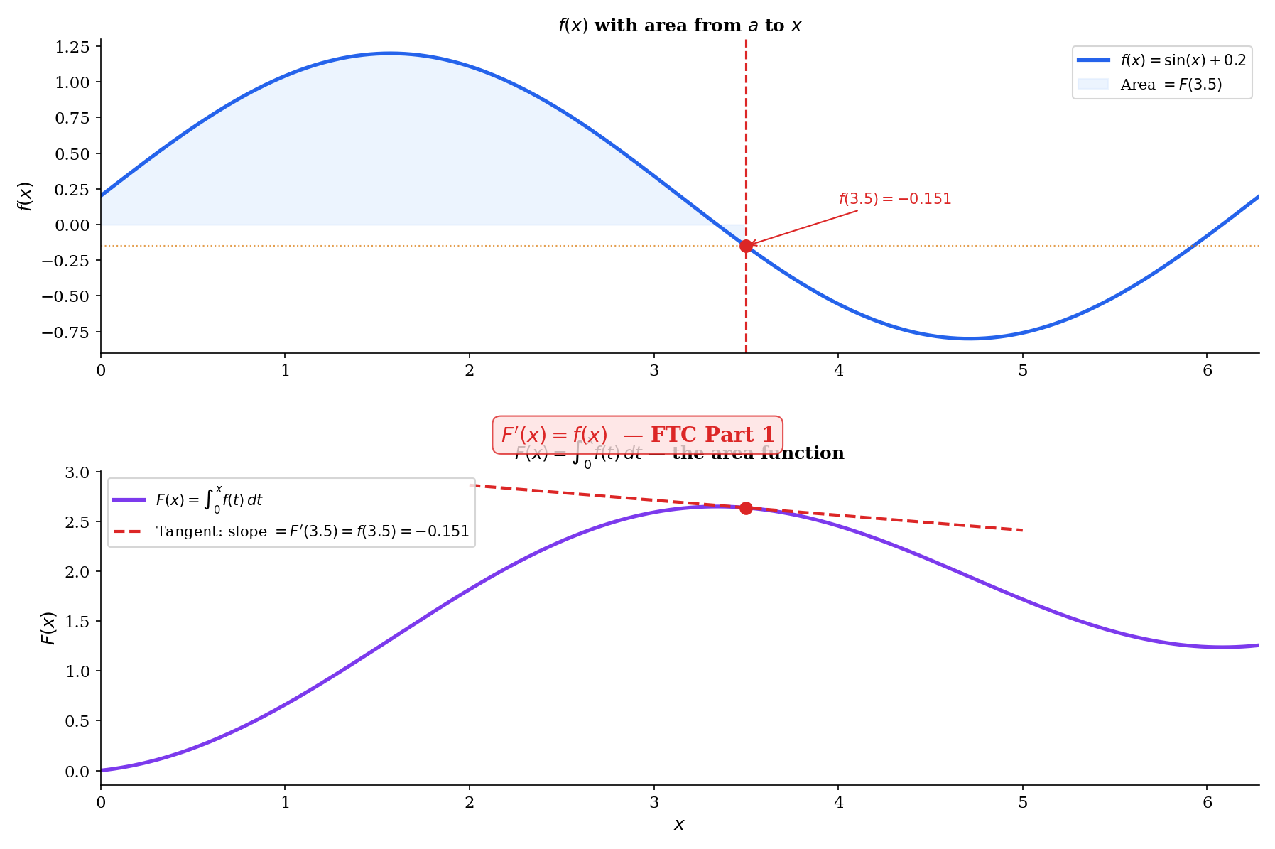
Consider the “area function” — the accumulated area under from to . As advances by a tiny amount , the area increases by approximately — a thin rectangle of height and width . So
The FTC Part 1 says this approximation is exact in the limit: . Differentiation undoes integration.
📐 Definition 5 (Antiderivative)
A function is an antiderivative of on if for all .
If is an antiderivative of , then so is for any constant — and these are the only antiderivatives. This follows from Corollary 1 of the MVT (Mean Value Theorem & Taylor Expansion): if on , then is constant.
🔷 Theorem 4 (Fundamental Theorem of Calculus, Part 1)
If is continuous on , then the function defined by
is continuous on , differentiable on , and for all .
Proof.
Fix . For with , the additivity of the integral gives:
Since is continuous at : given , choose such that . For , every between and satisfies , so . Therefore:
The integral bound uses for all in the interval of length , and the triangle inequality for integrals (Theorem 3(d)).
This shows , i.e., .
📝 Example 5 (Differentiating an integral with no closed-form antiderivative)
No antiderivative of exists in elementary functions (the integral defines the Fresnel function ). But the FTC Part 1 tells us the derivative of the area function anyway. This illustrates the power of FTC1: we can differentiate integrals even when we cannot compute them in closed form.
📝 Example 6 (Chain rule version of FTC1)
Here the upper limit is rather than itself. By the chain rule (The Derivative & Chain Rule, Theorem 6): if , then by FTC1, and .
The Fundamental Theorem of Calculus, Part 2
FTC Part 1 tells us that every continuous function has an antiderivative (namely ). FTC Part 2 tells us how to use an antiderivative to compute a definite integral: evaluate at the endpoints and subtract.
🔷 Theorem 5 (Fundamental Theorem of Calculus, Part 2)
If is continuous on and is any antiderivative of on (i.e., for all ), then
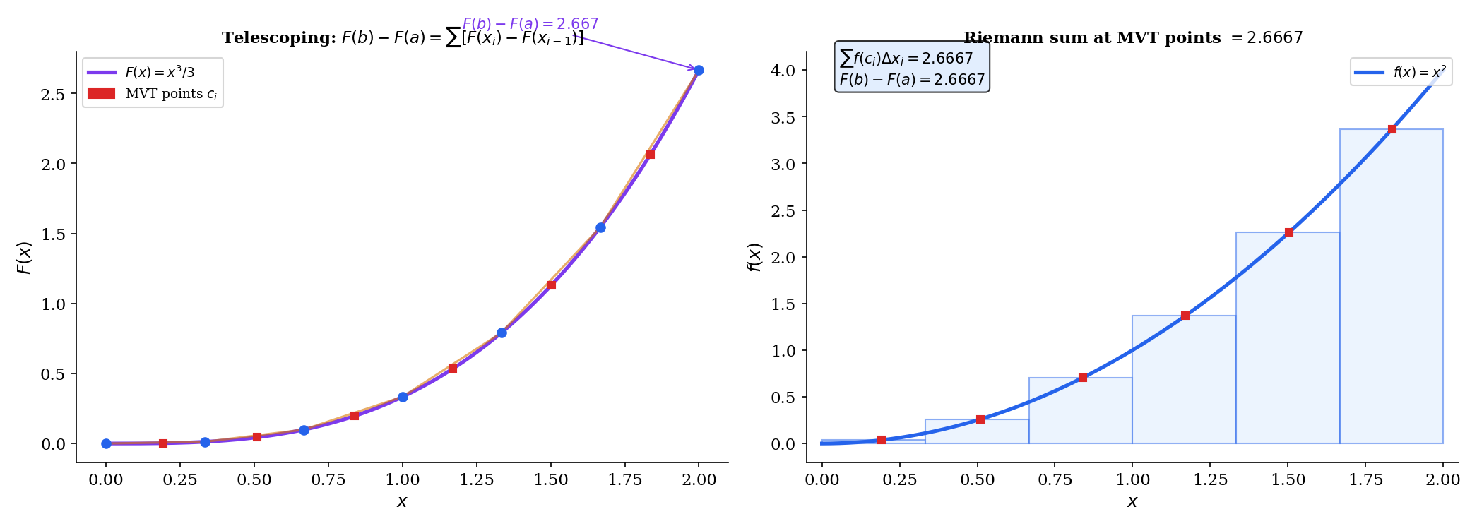
Proof.
Let be any partition of . Write as a telescoping sum:
By the Mean Value Theorem (Mean Value Theorem & Taylor Expansion, Theorem 2), applied to on each subinterval : there exists such that
So the telescoping sum becomes a Riemann sum:
Since is continuous (hence Riemann integrable by Theorem 1), as every Riemann sum converges to . But the left side is independent of the partition. Therefore:
📝 Example 7 (∫₀¹ x² dx via FTC2)
Compare with Example 3: the same answer, in one line instead of a page of algebra. The FTC transforms a limit evaluation into an antiderivative evaluation.
📝 Example 8 (∫₀π sin(x) dx)
The area under one arch of the sine curve is exactly 2.
💡 Remark 4 (The two parts of FTC are not converses)
Part 1 says: start with continuous construct get . Part 2 says: start with any antiderivative of . They are complementary, not equivalent. Part 1 is an existence result (continuous functions have antiderivatives); Part 2 is a computation result (integrals can be evaluated via antiderivatives).
Integration Techniques
🔷 Theorem 6 (Substitution Rule (Change of Variables))
If is continuously differentiable and is continuous on the range of , then
Proof.
Let be an antiderivative of (exists by FTC Part 1 since is continuous). Then by the chain rule (The Derivative & Chain Rule, Theorem 6):
So is an antiderivative of . By FTC Part 2:
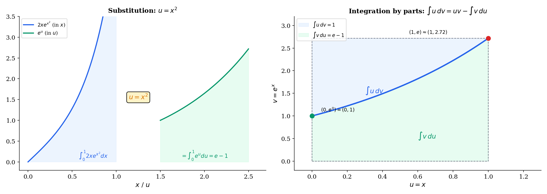
📝 Example 9 (∫₀¹ 2x e^(x²) dx)
Let , so . The bounds transform: , . Therefore:
🔷 Theorem 7 (Integration by Parts)
If and are continuously differentiable on , then
Proof.
By the product rule (The Derivative & Chain Rule, Theorem 4): . Integrate both sides from to using FTC Part 2:
Rearrange to get the integration by parts formula.
📝 Example 10 (∫₀¹ x eˣ dx)
Let and , so and . Then:
💡 Remark 5 (The chain rule and product rule in reverse)
Substitution is the chain rule read from right to left. Integration by parts is the product rule rearranged. Every differentiation rule has an integration counterpart — they are the same theorems, applied in opposite directions.
The Integral Form of the Taylor Remainder
This section resolves the forward reference from Mean Value Theorem & Taylor Expansion, Remark 4, which stated the integral remainder without proof.
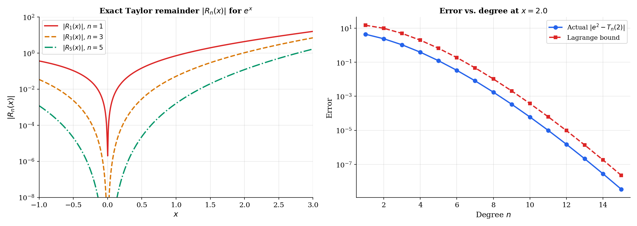
🔷 Theorem 8 (Integral Remainder for Taylor's Theorem)
If is -times continuously differentiable on an interval containing and , then
where the remainder is given by
Proof.
By induction on .
Base case (): We need . This is exactly FTC Part 2 applied to : .
Inductive step: Assume the result holds for :
Apply integration by parts with
Then:
Evaluating the boundary term: at , ; at , the term is . So:
Absorbing into the Taylor polynomial of degree gives the result.
💡 Remark 6 (Lagrange remainder from the integral remainder)
The Lagrange form (from Mean Value Theorem & Taylor Expansion, Theorem 4) follows from the integral form by the Mean Value Theorem for Integrals. The integral form is stronger: it gives the exact remainder as an integral, not just a bound involving an unknown intermediate point .
Numerical Integration
When antiderivatives don’t exist in closed form — which is most of the time in practice — we compute integrals numerically. The Riemann sum framework we’ve developed is not just a theoretical tool; it’s the blueprint for computational quadrature.
🔷 Proposition 3 (Error Bounds for Quadrature Rules)
For with sufficient smoothness on with subintervals of width :
(a) Left/Right endpoint rule: — error .
(b) Trapezoidal rule: — error .
(c) Simpson’s rule: — error .
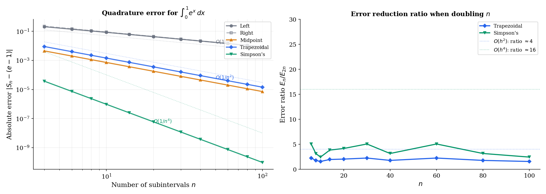
📝 Example 11 (Error comparison across quadrature rules)
Approximate with subintervals:
| Rule | Approximation | | Bound | |------|---------------|-----------|-------| | Left | | | | | Trapezoidal | | | | | Simpson’s | | | |
Simpson’s rule achieves 6 digits of accuracy with just 10 subintervals. The convergence rates — , , — explain why higher-order methods dominate in practice.
💡 Remark 7 (Simpson's rule and polynomial interpolation)
Simpson’s rule fits a parabola through every three consecutive points , , , then integrates the parabola exactly. It is exact for polynomials up to degree 3 — not just degree 2 — because of a symmetry cancellation. This is why the error involves , not .
Connections to Statistics
The Riemann integral is the analytical engine for every probabilistic computation involving a continuous distribution. Densities, expectations, moments, posteriors — they are integrals.
Expectation as an integral
is the defining integral of probability. Variance, covariance, and all moments are expected values, hence all are integrals; the linearity, monotonicity, and additivity properties developed here are the algebraic foundations of moment computations. See formalStatistics Expectation & Moments.
Likelihood and Fisher information
The expected log-likelihood is an integral over the data distribution. The score and Fisher information are integrals against the parameter-indexed density; integration by parts and differentiation under the integral sign drive the asymptotic theory of maximum likelihood. See formalStatistics Maximum Likelihood.
Bayesian posteriors as integrals
The posterior has an integral normalizing constant. Bayesian estimators, credible intervals, and posterior predictives are all posterior expectations. MCMC is fundamentally an integral-approximation method for cases when the closed form fails. See formalStatistics Bayesian Computation & MCMC.
Connections to ML
The integral is one of the most ubiquitous operations in machine learning — arguably more so than the derivative, since every expected value, every probability computation, and every marginal distribution involves integration.
Expected values as integrals
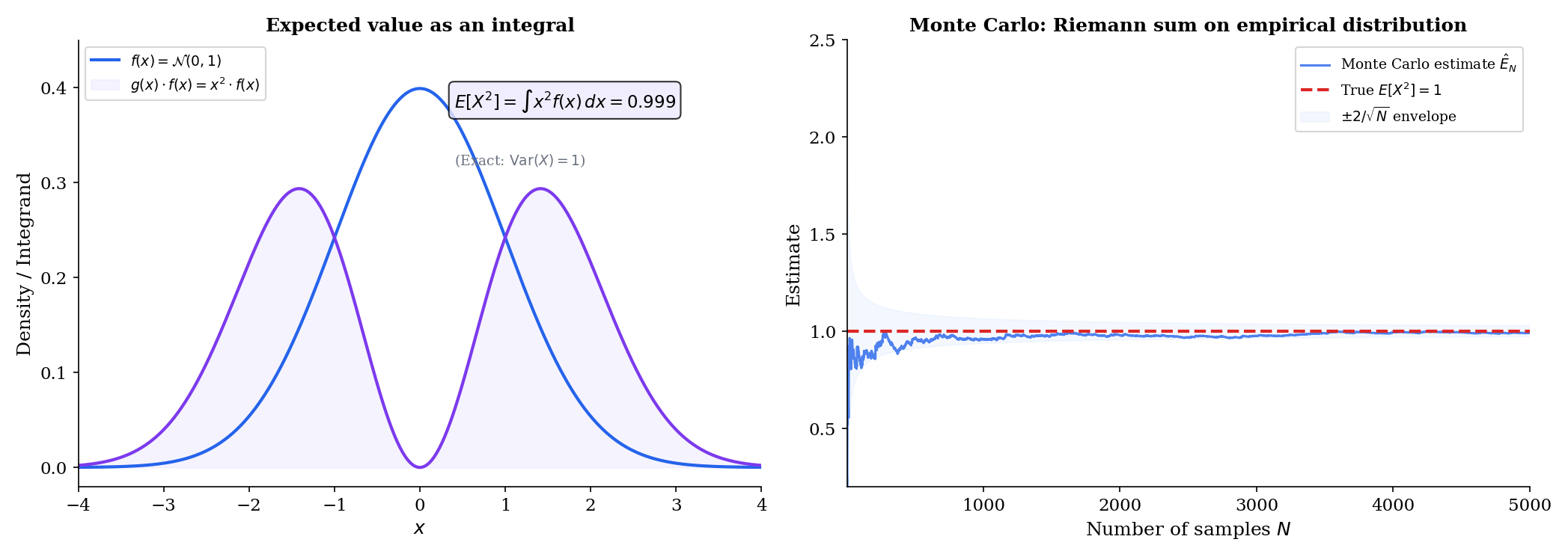
If is a continuous random variable with density , then the expected value of any function is
The risk (expected loss) of a hypothesis is . We can’t compute this integral exactly (we don’t know ), so we approximate it with the empirical risk: . This is literally a Riemann sum — the Monte Carlo approximation replaces the integral with a finite sum over data points.
→ Measure-Theoretic Probability on formalML
Marginalizing over latent variables
Mixture models define — the observed density is obtained by integrating over the latent variable . Variational autoencoders work with . When this integral is intractable (it almost always is in high dimensions), we resort to variational lower bounds (the ELBO) or numerical quadrature.
→ Bayesian Nonparametrics on formalML
Information-theoretic quantities
Entropy, KL divergence, and cross-entropy are all integrals over densities:
The properties of the integral — linearity, monotonicity — directly yield Gibbs’ inequality () and other fundamental information-theoretic bounds.
→ Shannon Entropy on formalML
Numerical quadrature in practice
When closed-form antiderivatives don’t exist, we compute integrals numerically. For 1D integrals, the trapezoidal and Simpson’s rules from §10 are effective. scipy.integrate.quad uses adaptive Gaussian quadrature — choosing subinterval sizes based on local function behavior, exactly the kind of partition refinement we studied in §2. For high-dimensional integrals (), Monte Carlo methods replace deterministic quadrature, because the curse of dimensionality makes grid-based methods impractical.
From Riemann to Lebesgue: why the generalization matters
The Riemann integral handles continuous and piecewise-continuous functions on bounded intervals. But ML requires more:
- Unbounded domains: (every expected value over ).
- Pathological functions: Indicator functions, densities with heavy tails, functions with uncountably many discontinuities.
- Exchanging limits and integrals: The dominated convergence theorem lets us pass limits inside integrals under mild conditions — essential for proving that the empirical risk converges to the true risk.
The Lebesgue integral handles all of these. The transition Riemann Lebesgue is the transition from introductory to measure-theoretic probability.
→ Measure-Theoretic Probability on formalML
Connections & Further Reading
Prerequisites — topics you need first
Sequences, Limits & Convergence
The Riemann integral is defined as a limit — specifically, the limit of Riemann sums as the partition mesh tends to zero. The convergence theory from Topic 1 provides the framework: the sequence of Riemann sums converges, and the integral is its limit.
Epsilon-Delta & Continuity
Integrability of continuous functions relies on uniform continuity, which was characterized via the ε-δ framework in Topic 2. The proofs of integrability criteria and the FTC use ε-δ arguments throughout.
Mean Value Theorem & Taylor Expansion
The FTC Part 2 proof uses the Mean Value Theorem: F(xᵢ) - F(xᵢ₋₁) = F'(cᵢ)(xᵢ - xᵢ₋₁) = f(cᵢ)Δxᵢ converts the telescoping sum into a Riemann sum. The integral form of the Taylor remainder, stated without proof in Topic 6 Remark 4, is proved here using integration by parts.
The Derivative & Chain Rule
The FTC connects differentiation and integration as inverse operations. The substitution rule is the chain rule in reverse; integration by parts is the product rule in reverse. The derivative definition from Topic 5 is essential throughout.
Completeness & Compactness
The proof that continuous functions on [a,b] are Riemann integrable uses the Heine-Cantor theorem: continuous functions on compact sets are uniformly continuous. Compactness of [a,b] (Heine-Borel, Topic 3) is the hidden engine behind integrability.
Where this leads — next in formalCalculus
Improper Integrals & Special Functions
Multiple Integrals & Fubini's Theorem
Fourier Series & Orthogonal Expansions
Approximation Theory
Sigma-Algebras & Measures
On to formalStatistics — where this calculus powers inference
Expectation Moments
The expected value E[g(X)] = ∫ g(x) f(x) dx is the defining integral of probability. Variance, covariance, and all moments are expected values — hence all are integrals. The linearity and monotonicity of the Riemann integral are the algebraic foundations of moment computations.
Maximum Likelihood
The expected log-likelihood E[log f(X|θ)] = ∫ log f(x|θ) · f(x|θ_0) dx is an integral; the score and Fisher information involve integrals over the parameter-indexed density. Integration by parts and differentiation under the integral sign drive the asymptotic theory.
Bayesian Computation And MCMC
The posterior p(θ|x) = p(x|θ)π(θ) / ∫ p(x|θ)π(θ) dθ has an integral normalizing constant. Bayesian estimators, credible intervals, and posterior predictives are all posterior expectations — hence integrals. MCMC is fundamentally an integral-approximation method.
Sufficient Statistics
The Fisher–Neyman factorization theorem L(θ; x) = g(T(x), θ) · h(x) is an identity about how the likelihood (an integrand) factors through the sufficient statistic. Establishing sufficiency in continuous models requires integrating the conditional density and verifying that θ drops out — a Riemann/Lebesgue integration argument.
Confidence Intervals And Duality
Topic 19's coverage probability P_θ(θ ∈ C(X)) is an integral of the sampling density over the event {θ ∈ C(X)}; §19.8 computes this integral numerically for the binomial-p coverage diagnostic.
Hypothesis Testing
Topic 17's size and power are integrals of the sampling density over the rejection region R: P_{H_0}(R) ≤ α defines size, β(θ) = ∫_R f(x; θ) dx is the power function. Differentiating β(θ) treats it as a calculus-of-variations object in θ.
Large Deviations
Topic 12's MGF M(t) = ∫ e^{tx} f(x) dx is an expectation integral, and the Cramér rate function I(x) = sup_t(tx − log M(t)) involves a supremum over an integral expression — the Legendre dual of the cumulant generating function.
Law Of Large Numbers
Topic 10's Khintchine and Etemadi SLLN proofs use the dominated convergence theorem in their truncation arguments: E[X_1 · 𝟙(|X_1| ≤ n)] → E[X_1] as n → ∞, with |X_1| as the dominating integrable function — a textbook DCT application.
Likelihood Ratio Tests And Np
Topic 18's Neyman–Pearson lemma proof integrates (φ* − φ)(f_1 − k f_0) ≥ 0 over the sample space to convert a pointwise inequality into an expectation inequality. §18.9's non-central χ² series sums integrals against shifted-df Gamma densities.
Modes Of Convergence
Topic 9 defines L^p convergence via the integral norm E[|X_n − X|^p] = ∫|X_n − X|^p dP; the dominated convergence theorem is used to interchange limits and integrals in the proof that L^p convergence implies convergence in probability.
Point Estimation
Topic 13's CRLB regularity conditions require interchange of derivative and integral: ∂/∂θ ∫ f(x; θ) dx = ∫ ∂_θ f(x; θ) dx. Dominated convergence justifies the swap; the resulting Fisher-information identity is the foundation of efficient estimation.
On to formalML — where this calculus powers ML
Measure Theoretic Probability
The Riemann integral defines expected values for continuous densities: E[X] = ∫ x f(x) dx. But Riemann integration fails for pathological functions like the indicator of the rationals. The Lebesgue integral, built on measure theory, resolves these limitations and is the foundation of rigorous probability theory.
Shannon Entropy
Differential entropy h(X) = -∫ f(x) log f(x) dx, KL divergence D_KL(p‖q) = ∫ p(x) log(p(x)/q(x)) dx, and cross-entropy are all defined as integrals. The properties of the integral — linearity, monotonicity, additivity — directly yield information-theoretic inequalities.
Bayesian Nonparametrics
Posterior computation requires integrating likelihood × prior over the parameter space. When conjugacy is unavailable, numerical quadrature (trapezoidal, Simpson's, Gaussian quadrature) provides the computational backbone. Understanding integration error bounds from this topic informs the accuracy of these approximations.
References
- book Abbott (2015). Understanding Analysis Chapter 7 develops the Riemann integral via the Darboux approach with exceptional clarity — our primary reference for the definition and integrability proofs
- book Rudin (1976). Principles of Mathematical Analysis Chapter 6 on Riemann-Stieltjes integration — the definitive compact treatment, though we specialize to the Riemann case
- book Spivak (2008). Calculus Chapters 13–14 develop integration with unmatched geometric motivation alongside full rigor — the best reference for the geometric intuition behind partitions and area
- book Folland (1999). Real Analysis Chapter 2 gives the Lebesgue integral — useful for understanding where Riemann fails and why the generalization matters
- book Burden & Faires (2010). Numerical Analysis Chapter 4 on numerical integration — trapezoidal rule, Simpson's rule, Gaussian quadrature error analysis