Approximation Theory
Every continuous function on a closed interval can be uniformly approximated by polynomials — the Weierstrass theorem. Bernstein polynomials provide the constructive proof, Chebyshev polynomials provide the optimal nodes, and Jackson's theorem quantifies how smoothness controls the rate. This is the existence theorem of approximation: the guarantee that good approximants exist, the machinery to build them, and the connection to the universal approximation theorem for neural networks.
Abstract. The Weierstrass approximation theorem guarantees that every continuous function f on a closed interval [a,b] can be uniformly approximated by polynomials: for any ε > 0, there exists a polynomial p with ||f − p||∞ < ε. The Bernstein polynomial construction Bₙ(f; x) = Σ f(k/n)C(n,k)xᵏ(1−x)ⁿ⁻ᵏ provides a concrete, constructive proof — each Bₙ is the expected value of f evaluated at a binomial random variable, and convergence follows from the law of large numbers. The convergence rate O(1/√n) is slow, but the theorem's power lies in its generality: no differentiability, no analyticity, just continuity. The Stone-Weierstrass theorem generalizes to compact spaces: a closed subalgebra of C(K) that separates points and contains the constants is dense. For optimal polynomial approximation, Chebyshev polynomials Tₙ(x) = cos(n arccos x) provide near-minimax approximation and the ideal interpolation nodes, avoiding the Runge phenomenon that plagues equispaced interpolation. Jackson's theorem quantifies the rate of best approximation: Eₙ(f) ≤ C·ω(f; 1/n), where ω is the modulus of continuity — smoother functions admit faster polynomial approximation. Bernstein's inverse theorem provides the converse: fast approximation implies smoothness. In machine learning, the universal approximation theorem for neural networks (Cybenko, Hornik) is the direct analog of Weierstrass: single-hidden-layer networks can uniformly approximate any continuous function on a compact set. Barron's theorem gives approximation rates for networks, and polynomial approximation underlies homomorphic encryption for private ML inference.
1. Overview & Motivation — Why Approximation Theory?
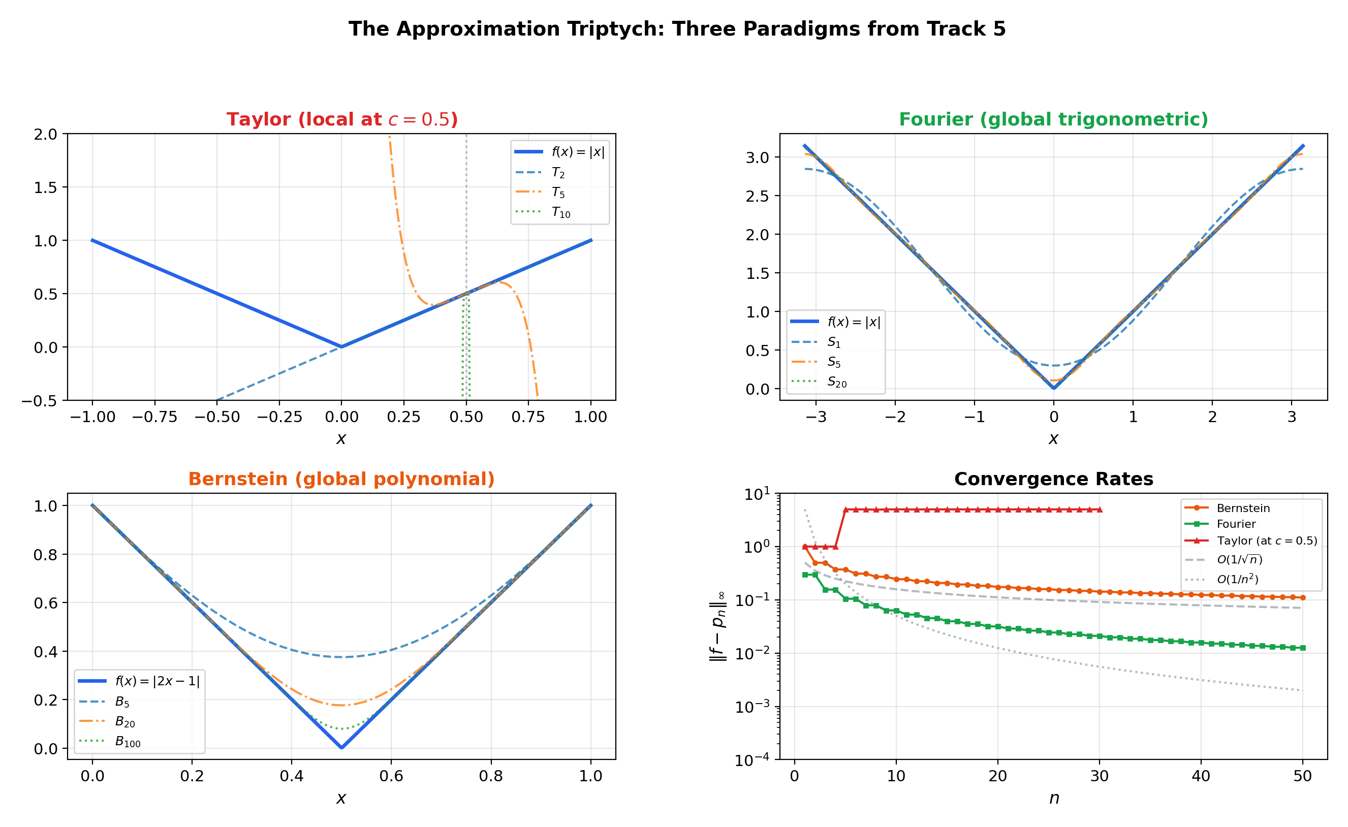
Track 5 has now developed three approximation paradigms. Power Series & Taylor Series showed how to approximate a function locally by matching derivatives at a center — but Taylor series require analyticity and are limited by the radius of convergence. Fourier Series & Orthogonal Expansions showed how to approximate a function globally by decomposing it into trigonometric harmonics — but Fourier series work best for periodic functions and converge in the norm, which allows large pointwise errors on small sets.
The capstone question of this track is: can we approximate any continuous function on by polynomials, uniformly (with a guaranteed pointwise bound everywhere)? The answer is yes — the Weierstrass approximation theorem — and understanding why, how, and how fast is the subject of approximation theory.
Why this matters in ML. The universal approximation theorem for neural networks (Cybenko 1989) is the neural-network analog of Weierstrass. Just as Weierstrass says polynomials are dense in , Cybenko says single-hidden-layer networks are dense in for compact . Understanding the classical theory illuminates the modern one — including its limitations. Density says approximants exist but says nothing about how to find them or how many parameters are needed. The gap between existence and computation is the gap between Weierstrass and training a neural network.
💡 Remark 1 (The approximation triptych)
Track 5 has developed three approximation paradigms, each with its own strengths and limitations:
| Taylor (Topic 18) | Fourier (Topic 19) | Weierstrass/Bernstein (Topic 20) | |
|---|---|---|---|
| Basis | Monomials | Trig functions | Bernstein basis |
| Scope | Local (radius around center ) | Global on the period | Global on |
| Requires | Analyticity | Integrability | Continuity only |
| Convergence | Inside radius | norm; pointwise under conditions | Uniform on |
| Coefficients | Derivatives: | Integrals: | Samples: |
Each successive paradigm trades specificity for generality. The thread connecting them all is the question: how well can we approximate functions, and what determines the answer?
2. The Weierstrass Approximation Theorem
The Weierstrass approximation theorem (1885) is the existence theorem of approximation theory. It tells us that polynomial approximation is always possible for continuous functions — the polynomials are dense in .
📐 Definition 1 (Best Polynomial Approximation)
For and , the best polynomial approximation error (or minimax error) of degree is
where is the space of polynomials of degree . The infimum is attained — compactness of , continuity of , and finite dimension of guarantee the existence of a best approximant with .
🔷 Theorem 1 (The Weierstrass Approximation Theorem)
If is continuous, then for every there exists a polynomial such that
Equivalently, as .
In the language of metric spaces: the polynomials are dense in .
💡 Remark 2 (What Weierstrass does and does not say)
The theorem is an existence result. It guarantees that good polynomial approximants exist but does not:
- Construct the best polynomial for a given
- Specify what degree is needed
- Identify the optimal polynomial
The Bernstein construction (Section 3) provides an explicit sequence of polynomial approximants. The Chebyshev theory (Section 6) characterizes the best approximant. Jackson’s theorem (Section 7) quantifies the rate.
3. Bernstein Polynomials — The Constructive Proof
The Bernstein polynomial is the simplest constructive proof of Weierstrass. It builds polynomial approximants by averaging over a binomial distribution — a probabilistic construction that converts the law of large numbers into an approximation theorem.
📐 Definition 2 (Bernstein Polynomial)
For and , the th Bernstein polynomial of is
The Bernstein basis polynomials are
These form a partition of unity: for all .
💡 Remark 3 (The probabilistic interpretation)
Let . Then
Each Bernstein polynomial evaluates at the random points weighted by the binomial probabilities. As , the law of large numbers gives in probability, so by continuity, giving . This is the heuristic — the rigorous proof makes it precise.
🔷 Theorem 2 (Uniform Convergence of Bernstein Polynomials)
If is continuous, then uniformly on :
Proof.
The proof uses three identities for the Bernstein basis:
Identity 1 (partition of unity): .
Identity 2 (first moment): .
Identity 3 (variance): .
Now fix . Since is continuous on the compact set , it is uniformly continuous: choose such that whenever .
For any , using Identity 1:
Split the sum into two parts. Let .
Near terms (): Here , so these terms contribute at most .
Far terms (): Here , and by Identity 3:
These terms contribute at most .
Combining: .
Choose . Then for all , so .
Since was arbitrary, uniformly.
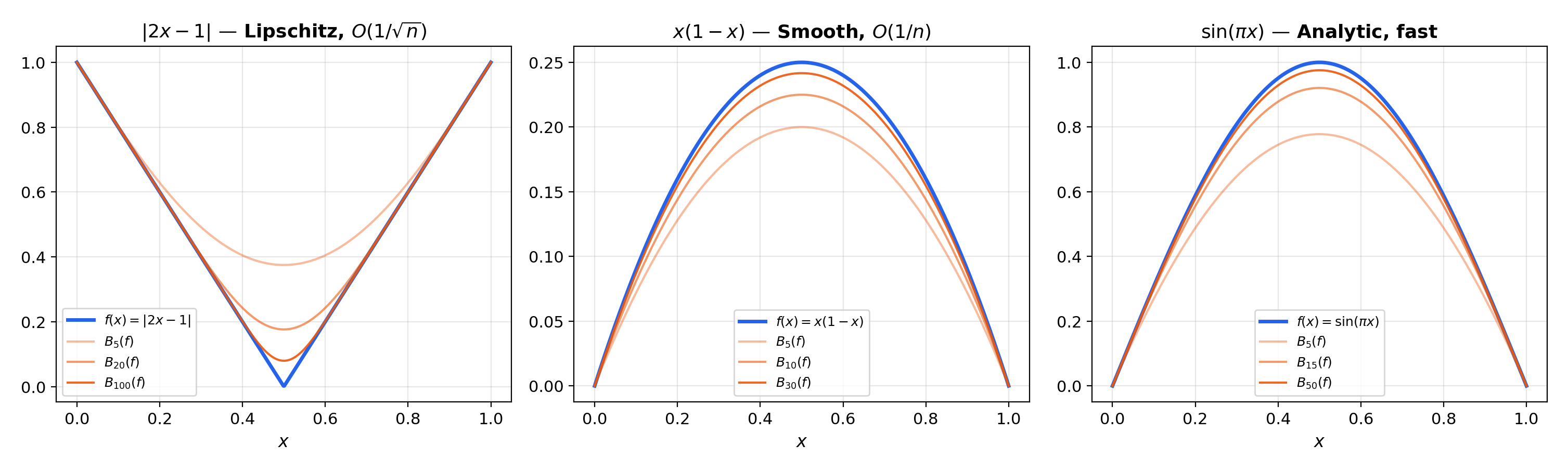
📝 Example 1 (Bernstein polynomials for f(x) = |2x − 1|)
The function is continuous but not differentiable at . Its Bernstein polynomials are smooth polynomials that converge uniformly to , rounding the corner at . At , the approximation is visibly smooth; at , it is nearly indistinguishable from except in a narrow region around .
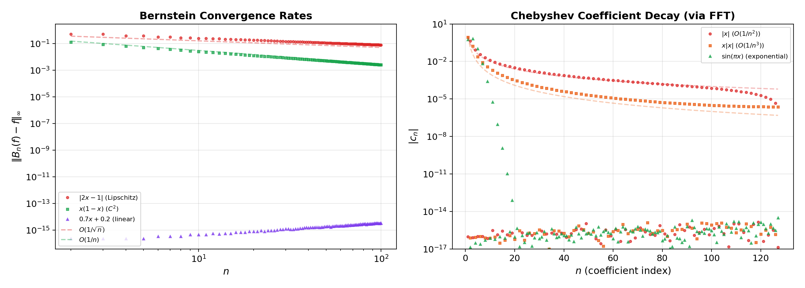
📝 Example 2 (Convergence rate comparison)
For the smooth function , the Bernstein polynomial satisfies , giving — faster than the general because is smooth.
For (Lipschitz but not ), — the worst-case rate for Lipschitz functions.
This illustrates that Bernstein convergence is slow — adequate for proving the Weierstrass theorem, but not optimal for computation.
4. Stone-Weierstrass — The Grand Generalization
Stone’s generalization (1937, 1948) replaces the specific polynomial algebra on with an abstract algebra on a compact space, identifying exactly what properties an algebra needs to be dense in .
📐 Definition 3 (Separating Algebra)
A set is a subalgebra of if it is closed under addition, scalar multiplication, and pointwise multiplication. separates points if for any in , there exists with . vanishes nowhere if for every , there exists with . If contains the constant functions, it automatically vanishes nowhere.
🔷 Theorem 3 (The Stone-Weierstrass Theorem (Real Version))
Let be a compact metric space and let be a subalgebra that separates points and contains the constant functions. Then is dense in under the sup-norm:
📝 Example 3 (Recovering the Weierstrass theorem)
Take and , the polynomials. Polynomials form a subalgebra (closed under , , scalar multiplication). They separate points: distinguishes any . They contain the constants. Therefore by Stone-Weierstrass. This is precisely Theorem 1.
📝 Example 4 (Trigonometric polynomials on the circle)
Take (the circle) and the trigonometric polynomials. They form a subalgebra (products of trig functions are trig functions), separate points (if then or ), and contain the constants. Stone-Weierstrass gives density, consistent with the Fourier series theory from Topic 19, which proved this concretely via Parseval’s identity.
📝 Example 5 (Polynomials in several variables)
Take compact and the polynomials in variables. They separate points: the coordinate functions distinguish points that differ in any coordinate. Stone-Weierstrass gives the density of multivariate polynomials in — a result that would be laborious to prove directly but follows immediately from the abstract theorem.
💡 Remark 4 (What Stone-Weierstrass does not cover)
The theorem applies to with the sup-norm. It does not directly apply to spaces (which require measure theory) or to non-compact domains (which require additional decay conditions). The complex version requires to be self-conjugate: . This condition is automatic for real-valued algebras but must be checked for complex ones.
![Three instances of Stone-Weierstrass — polynomials on [0,1], trigonometric polynomials on the circle, multivariate polynomials on a compact subset of R²](/images/topics/approximation-theory/stone-weierstrass-examples.png)
5. Best Approximation — vs. Uniform
The choice of norm changes the best approximant, the characterization of optimality, and the connection to other mathematical structures. Two norms, two optimization problems, two different answers.
📐 Definition 4 (Best Approximation in L² and C)
The best approximation of from is the polynomial minimizing
The best uniform (Chebyshev) approximation of from is the polynomial minimizing
🔷 Theorem 4 (Best L² Approximation as Orthogonal Projection)
The best polynomial approximation is the orthogonal projection of onto in the inner product . If is an orthonormal basis for (e.g., the Legendre polynomials), then
This is exactly the Fourier coefficient formula from Topic 19, with orthogonal polynomials replacing trigonometric functions.
💡 Remark 5 (L² vs. uniform — why both matter)
best approximation is easy to compute (orthogonal projection — just compute inner products) but allows large pointwise errors on small sets. Uniform best approximation is hard to compute (a nonlinear optimization problem) but gives a guaranteed pointwise bound everywhere.
In ML: approximation corresponds to minimizing mean squared error (training loss), while uniform approximation corresponds to worst-case guarantees (robustness). A model that minimizes MSE can still have catastrophic errors on rare inputs — the gap between and uniform approximation is the gap between average-case and worst-case performance.
📝 Example 6 (Comparing L² and uniform best approximation of |x|)
For on with (quadratic approximation): the best approximant is the orthogonal projection (computed from Legendre coefficients), while the best uniform approximant has an equioscillation property — the error alternates between and at three points. The two approximants are different polynomials — the norm determines the answer.
![L² vs. uniform best quadratic approximation of |x| on [-1,1], showing equioscillation for the uniform approximant](/images/topics/approximation-theory/best-approximation-comparison.png)
6. Chebyshev Polynomials & Optimal Nodes
Chebyshev polynomials are the algebraic analog of the trigonometric functions — they arise from , connect polynomial approximation to Fourier analysis, and provide the optimal interpolation nodes.
📐 Definition 5 (Chebyshev Polynomials)
The Chebyshev polynomial of the first kind is
Equivalently, is the unique polynomial of degree with leading coefficient (for ) satisfying for .
The zeros are the Chebyshev nodes:
🔷 Theorem 5 (Chebyshev Minimax Property)
Among all monic polynomials of degree (leading coefficient ), the one with smallest sup-norm on is , and
achieved uniquely by the normalized Chebyshev polynomial.
🔷 Proposition 1 (The Equioscillation Theorem (Chebyshev's Theorem))
For , a polynomial is the best uniform approximation if and only if the error equioscillates at least times: there exist such that
(alternating sign, full magnitude). This characterizes the best approximant uniquely.
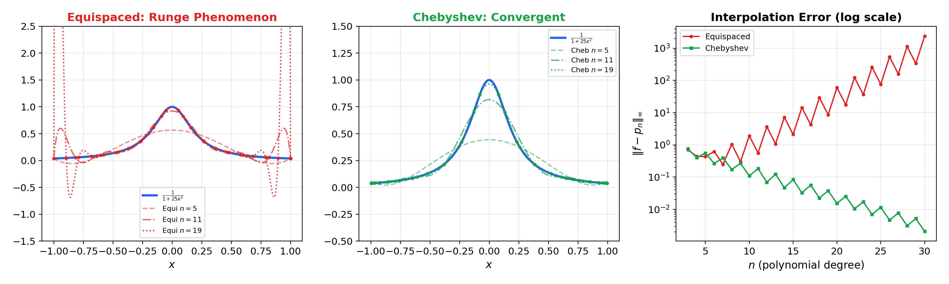
📝 Example 7 (The Runge phenomenon)
Consider interpolating on using polynomial interpolation. With equispaced nodes, the interpolant diverges near the endpoints as — the maximum interpolation error grows without bound. With Chebyshev nodes , the interpolant converges uniformly.
The Runge phenomenon is the polynomial interpolation analog of the Gibbs phenomenon from Topic 19: equispaced sampling is suboptimal, and the right node distribution matters enormously.
💡 Remark 6 (Chebyshev polynomials as 'cosines in disguise')
The identity means that Chebyshev approximation on is equivalent to Fourier cosine approximation on under the substitution . This connects Topic 20 back to Topic 19: the Chebyshev coefficients of are the Fourier cosine coefficients of , and the coefficient decay rates from Topic 19 translate directly into approximation rates for Chebyshev expansions.
7. Jackson’s Theorem & Bernstein’s Inverse
How fast can we approximate? Jackson’s theorem says the rate of best polynomial approximation is controlled by the smoothness of — smoother functions admit faster approximation. Bernstein’s inverse theorem gives the converse: fast approximation implies smoothness.
📐 Definition 6 (Modulus of Continuity)
The modulus of continuity of is
is Lipschitz (with constant ) if . is Hölder continuous with exponent if . The modulus quantifies “how continuous” is — it is the most refined scalar measure of regularity for continuous functions.
🔷 Theorem 6 (Jackson's Theorem (Direct Theorem))
If , then for every ,
where is an absolute constant. More generally, if (i.e., is times continuously differentiable), then
The smoother is, the faster .
🔷 Theorem 7 (Bernstein's Inverse Theorem)
If for some integer and , then and is Hölder continuous with exponent :
The converse of Jackson’s theorem: fast approximation rates imply smoothness.
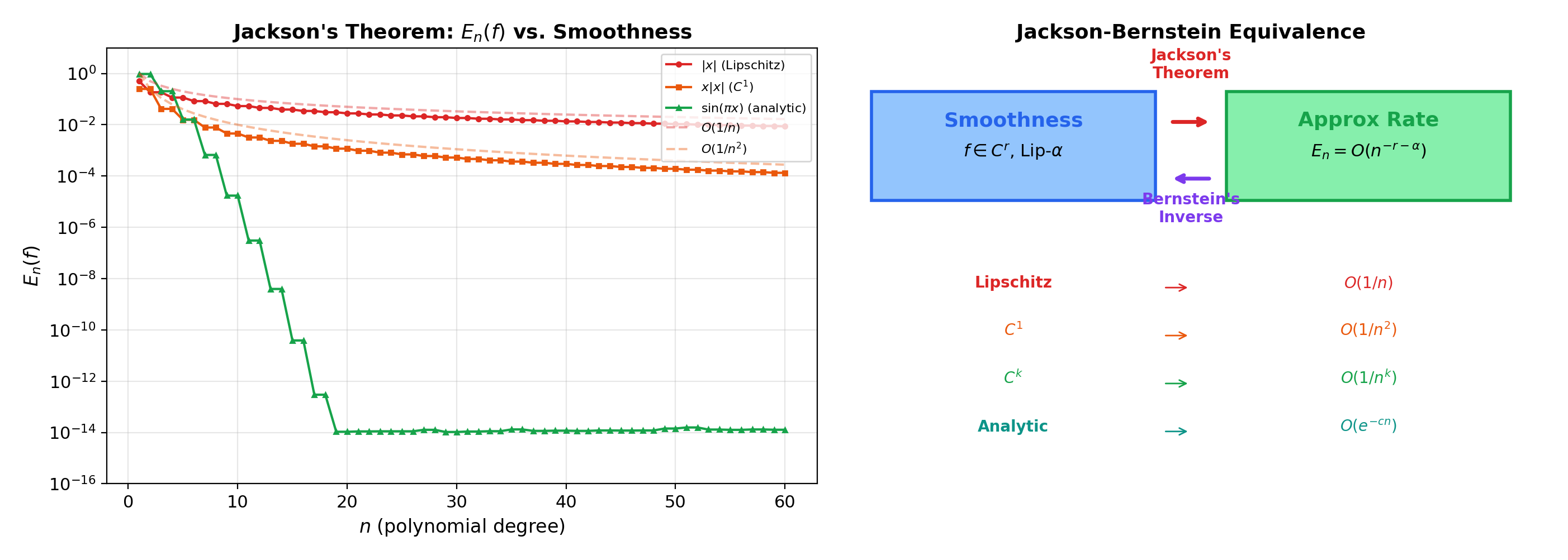
📝 Example 8 (Jackson's theorem for functions of varying smoothness)
(a) is Lipschitz (), so Jackson gives .
(b) is with Lipschitz derivative, so .
(c) (analytic) has — superalgebraic convergence.
This mirrors the Fourier coefficient decay hierarchy from Topic 19: the same smoothness conditions control both Fourier coefficient decay and polynomial approximation rates.
💡 Remark 7 (The Jackson-Bernstein equivalence)
Together, Jackson’s and Bernstein’s theorems establish that
Approximation rate and smoothness are two sides of the same coin. This tight equivalence has no analog in Fourier theory (where coefficient decay characterizes smoothness of periodic functions).
8. ML Connections — Universal Approximation, Barron’s Theorem, Private Inference
8.1 The universal approximation theorem
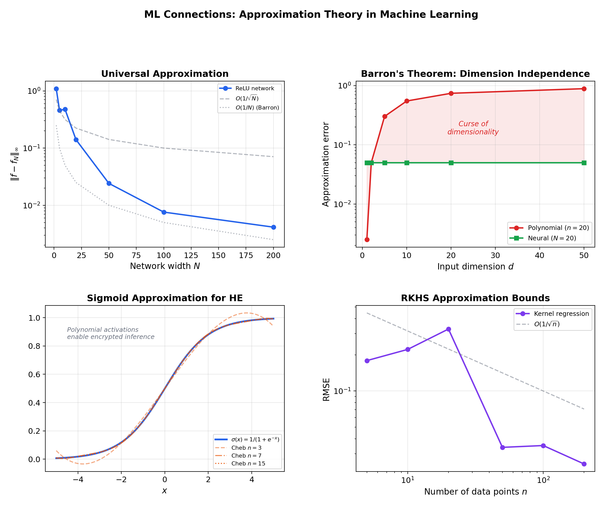
Cybenko (1989) and Hornik, Stinchcombe & White (1990) proved that single-hidden-layer networks with sigmoidal activation functions can uniformly approximate any continuous function on a compact set: the set
is dense in for compact . The proof structure mirrors Stone-Weierstrass: neural networks with a sigmoidal activation function form a set that separates points (by varying ), discriminates constants (by varying ), and is closed under the relevant operations.
The theorem says neural networks can approximate anything — but says nothing about how many neurons are needed. This is the same gap as in Weierstrass: existence without constructive bounds.
8.2 Barron’s theorem — approximation rates for networks
Barron (1993) proved a Jackson-type theorem for neural networks: if has bounded first-moment Fourier transform , then the best approximation by a network with hidden units satisfies
The rate is independent of the input dimension — this avoids the curse of dimensionality that plagues polynomial approximation in high dimensions (where Jackson’s theorem gives rates that degrade exponentially in ). This is why neural networks outperform polynomials for high-dimensional function approximation.
8.3 Polynomial approximation in homomorphic encryption
In privacy-preserving ML inference, computations on encrypted data must be polynomial — addition and multiplication only, no comparisons, no divisions. Activation functions like ReLU and sigmoid are approximated by low-degree polynomials (typically Chebyshev or Bernstein) so that inference can be performed on encrypted inputs.
Bernstein polynomials are particularly useful because they preserve the range : if , then — a property that sigmoid approximations need.
8.4 Kernel methods and RKHS approximation
In kernel-based ML (Gaussian processes, support vector machines), the function space is a reproducing kernel Hilbert space (RKHS). The representer theorem states that the best approximation in the RKHS from data points is a finite linear combination of kernel evaluations — an approximation-theoretic result. The RKHS approximation error depends on the RKHS norm of the target function, analogous to how depends on the smoothness of in Jackson’s theorem.
9. Computational Notes
-
Bernstein polynomial evaluation: Direct evaluation of is per point. The de Casteljau algorithm evaluates Bézier curves (which use the Bernstein basis) numerically stably via recursive linear interpolation.
-
Chebyshev expansion: For a function on , the Chebyshev coefficients can be computed via the FFT on the Chebyshev nodes (the discrete cosine transform). This gives all coefficients in operations — the same complexity as the FFT for Fourier coefficients.
-
Clenshaw’s algorithm evaluates a Chebyshev expansion in operations using the three-term recurrence , analogous to Horner’s method for monomial-form polynomials.
-
Numerical verification: The interactive visualization above lets you compare Bernstein polynomial approximation errors for (convergence rate ) and (convergence rate ). Verify Chebyshev vs. equispaced interpolation for Runge’s function .
10. Track 5 Completion
This topic completes the Sequences, Series & Approximation track. The four topics form a natural progression:
- Series Convergence & Tests — When do infinite sums converge? Absolute vs. conditional convergence, comparison and ratio tests.
- Power Series & Taylor Series — Local polynomial approximation from derivatives, radius of convergence, Taylor remainder.
- Fourier Series & Orthogonal Expansions — Global trigonometric approximation from integrals, orthogonality, coefficient decay, Gibbs phenomenon.
- Approximation Theory — The theoretical limits of polynomial approximation: existence (Weierstrass), construction (Bernstein), optimality (Chebyshev), rates (Jackson-Bernstein).
The thread connecting them all is the question: how well can we approximate functions, and what determines the answer?
Comparing three approximation methods
Connections & Further Reading
Prerequisites — topics you need first
Fourier Series & Orthogonal Expansions
Fourier partial sums are the best L² approximation among trigonometric polynomials (projection onto the trig subspace). Topic 20 asks: Can we do the same with algebraic polynomials? The answer is yes — the Weierstrass theorem — and the two approximation paradigms (L² vs. uniform, trig vs. polynomial) are unified by Stone-Weierstrass.
Uniform Convergence
The Weierstrass theorem is a statement about uniform convergence: Bₙ(f) → f uniformly on [0,1]. The proof uses the uniform continuity of f on compact sets (Topic 4, §3) and the uniform version of the law of large numbers. Stone-Weierstrass uses the lattice version of uniform closure.
Power Series & Taylor Series
Taylor polynomials give a local approximation at a center c, requiring analyticity for convergence. Bernstein polynomials provide a global approximation on [0,1] that requires only continuity. This is the central contrast: local + smooth vs. global + continuous. Topic 20 completes the approximation triptych: Taylor (local polynomial) → Fourier (global trigonometric) → Weierstrass (global polynomial).
The Riemann Integral & FTC
The L² best approximation norm ||f − p||₂ = √(∫(f−p)²dx) requires Riemann integration. Jackson's theorem uses the modulus of continuity ω(f; δ), which connects to uniform continuity on compact intervals. The Bernstein polynomial Bₙ(f; x) = E[f(Sₙ/n)] can be interpreted as an integration (expectation) against the binomial distribution.
Series Convergence & Tests
The convergence rate of Bernstein polynomials — ||Bₙ(f) − f||∞ = O(ω(f; 1/√n)) — involves series-like decay estimates. Jackson's theorem bounds the best-approximation error Eₙ(f) using techniques that parallel the convergence rate analysis from Topic 17.
Where this leads — next in formalCalculus
Metric Spaces & Topology
Density of polynomials in C[a,b] under the sup-norm is a statement about metric-space topology; the contraction mapping theorem sheds light on Bernstein operator iteration.
Normed & Banach Spaces
C[a,b] and L²[a,b] as Banach spaces; best approximation in normed spaces; the equioscillation theorem as a characterization in the dual space.
Inner Product & Hilbert Spaces
Best L² approximation as orthogonal projection; Legendre polynomials as an orthonormal basis; RKHS approximation theory.
Calculus of Variations
Best approximation as optimization over function spaces. The direct method provides the general existence principle.
On to formalStatistics — where this calculus powers inference
Kernel Density Estimation
KDE is a function-approximation problem — approximating the unknown density f by convolution with a kernel at bandwidth h. Consistency rates depend on the smoothness class of f (Hölder, Sobolev). Minimax rates for density estimation are approximation-theory results.
Empirical Processes
Bracketing numbers and covering numbers — approximation-theoretic measures of the 'size' of a function class — control the uniform convergence rate √n(P_n - P) over function classes. Donsker classes are exactly those whose bracketing integral converges.
Bootstrap
The bootstrap approximates the true sampling distribution of an estimator by the bootstrap sampling distribution. The validity proof is an approximation statement: the bootstrap empirical process converges to the same Gaussian limit as the true empirical process.
On to formalML — where this calculus powers ML
PAC Learning
The universal approximation theorem for neural networks (Cybenko 1989, Hornik 1991) is the neural-network analog of the Weierstrass theorem. The proof structure mirrors Stone-Weierstrass: networks form an algebra that separates points. Barron's theorem gives O(1/√n) approximation rates for networks with bounded first moments — the same rate as Bernstein polynomials.
Gradient Descent
Polynomial and Chebyshev approximation of activation functions enables private ML inference via homomorphic encryption. Bernstein polynomials preserve the bounded range [0,1], making them suitable for approximating sigmoid and ReLU in encrypted computation.
Spectral Theorem
The Stone-Weierstrass theorem for C*-algebras gives the continuous functional calculus: for self-adjoint operator A, f(A) is defined by approximating f with polynomials in A. This is the infinite-dimensional generalization of the polynomial approximation theory developed here.
Riemannian Geometry
RKHS approximation theory provides error bounds for kernel regression and Gaussian processes. The representer theorem is an approximation-theoretic result about best approximation in RKHS — the kernel analog of best polynomial approximation in C[a,b].
References
- book Rudin (1976). Principles of Mathematical Analysis Chapter 7 — the Stone-Weierstrass theorem and uniform approximation
- book Trefethen (2019). Approximation Theory and Approximation Practice The definitive modern treatment of Chebyshev approximation, interpolation, and practical polynomial approximation — the computational perspective
- book DeVore & Lorentz (1993). Constructive Approximation Chapters 1–4 — Bernstein polynomials, Jackson theorems, moduli of smoothness, inverse theorems
- book Abbott (2015). Understanding Analysis Chapter 6 — the Weierstrass approximation theorem via Bernstein polynomials, the cleanest undergraduate proof
- paper Cybenko (1989). “Approximation by Superpositions of a Sigmoidal Function” The original universal approximation theorem for neural networks — the neural-network Weierstrass theorem
- paper Hornik, Stinchcombe & White (1990). “Universal Approximation of an Unknown Mapping and Its Derivatives Using Multilayer Feedforward Networks” Extension of Cybenko's result to networks with arbitrary activation functions and derivative approximation