Inner Product & Hilbert Spaces
Adding angles and orthogonality to Banach spaces — from the projection theorem and Riesz representation through orthonormal bases and the spectral theorem to RKHS, kernel methods, and Gaussian processes.
Abstract. A normed space tells you how far apart points are, but not the angle between directions. An inner product adds angles, orthogonality, and projection — and these three geometric ideas unlock results of extraordinary power. The projection theorem guarantees that every point in a Hilbert space has a unique closest point in any closed convex subset. The Riesz representation theorem identifies a Hilbert space with its dual, collapsing the distinction between vectors and linear functionals. The spectral theorem decomposes compact self-adjoint operators into eigenspaces. And reproducing kernel Hilbert spaces provide the mathematical framework for every kernel method in machine learning — from SVMs through Gaussian processes to neural tangent kernels.
1. Overview and Motivation
In a reproducing kernel Hilbert space, evaluating a function at a point is an inner product: . This single identity — the reproducing property — is the engine behind SVMs, Gaussian processes, and kernel PCA. It works because is a Hilbert space, not just a Banach space. And it works because the inner product gives us something a norm alone cannot: angles.
A norm measures length. An inner product measures both length and angle. Angle gives you orthogonality; orthogonality gives you projection; projection gives you everything.
The arc of Track 8 is a staircase of abstraction, where each step adds one axiom and gains strictly stronger conclusions:
- Metric spaces (Topic 29): distances → completeness → fixed-point theorems.
- Normed/Banach spaces (Topic 30): length → bounded operators → Baire, UBP, Open Mapping, Closed Graph.
- Inner product/Hilbert spaces (this topic): angles → orthogonality → projection theorem, Riesz representation, spectral decomposition, RKHS.
Topic 31 is where the reader adds one more axiom and gains an enormous amount of power. Where Topic 30 was algebraic machinery — Baire-powered theorems, careful epsilon-management — this topic is geometric machinery. The proofs are more visual. The projection theorem is a “closest point” argument. The Riesz representation theorem is a “find the unique vector representing a functional” argument. The spectral theorem is an eigenvalue-decomposition argument. At every turn, the geometry of orthogonality does the heavy lifting.
2. Inner Product Spaces
📐 Definition 1 (Inner Product)
An inner product on a real vector space is a function satisfying:
- Symmetry: for all .
- Linearity in the first argument: for all and scalars .
- Positive definiteness: for all , with equality if and only if .
Every inner product induces a norm and hence a metric . A vector space equipped with an inner product is called an inner product space (or pre-Hilbert space).
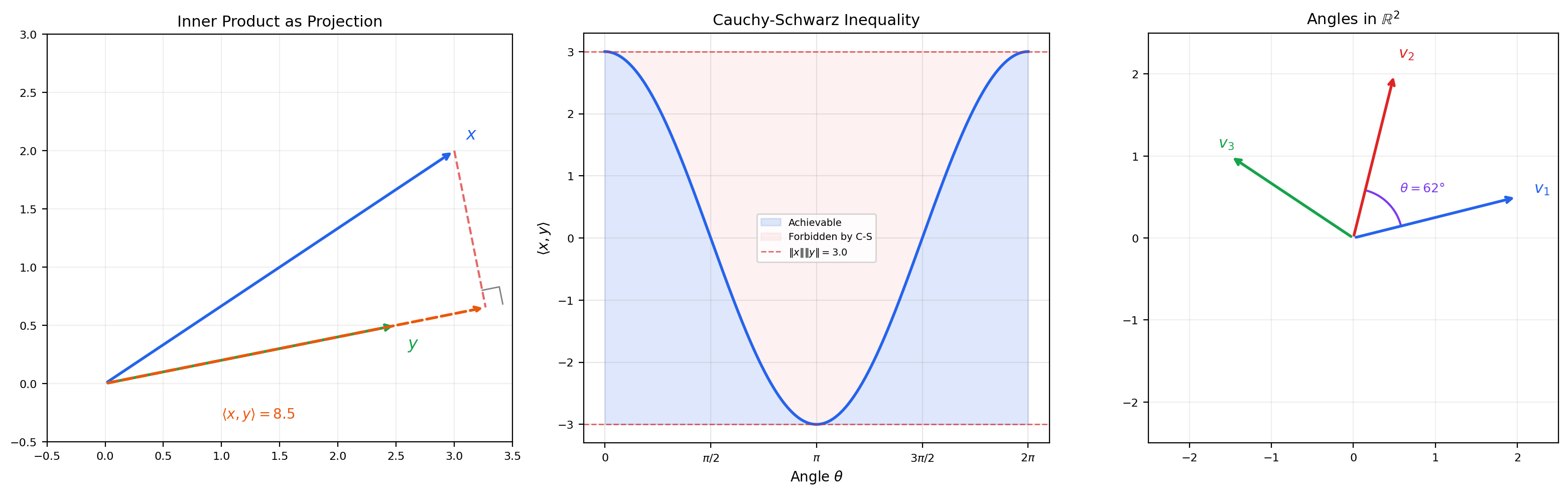
The inner product encodes geometry: the angle between nonzero vectors and is , and two vectors are orthogonal when . This is the geometric structure that a norm lacks.
📝 Example 1 (Euclidean Inner Product on ℝⁿ)
The standard inner product on is the dot product:
This induces the Euclidean norm . The angle formula recovers the geometric angle between vectors in and that we know from linear algebra.
📝 Example 2 (The L² Inner Product)
📝 Example 3 (The ℓ² Inner Product)
On the sequence space :
The series converges absolutely by Cauchy-Schwarz (Theorem 1 below). This is the discrete analog of the inner product — it is .
📝 Example 4 (Weighted Inner Products)
Given positive weights , the weighted inner product on is:
The induced norm stretches the geometry along coordinate axes. In machine learning, the Mahalanobis distance uses a weighted inner product where is a covariance matrix.
💡 Remark 1 (Banach Space Vocabulary Refresh)
If you completed Topic 30 some time ago, here is a brief refresher of the key definitions we will need. A normed space is a vector space with a norm satisfying positive definiteness, homogeneity, and the triangle inequality (Topic 30, Definition 1). A Banach space is a complete normed space (Topic 30, Definition 2). A bounded linear operator satisfies for some constant (Topic 30, Definition 3). The dual space is the space of all bounded linear functionals (Topic 30, Section 10). Every inner product space is a normed space (via ), and the Hilbert-space inner product will simplify the dual-space machinery of Topic 30 dramatically.
3. Cauchy-Schwarz and the Parallelogram Law
These are the two fundamental identities that govern inner product spaces. Every further result in this topic depends on one or both of them.
🔷 Theorem 1 (Cauchy-Schwarz Inequality)
For any vectors in an inner product space:
Equality holds if and only if and are linearly dependent.
Proof.
If , both sides are zero. Assume . For any , the positive definiteness of the inner product gives:
This is a quadratic in that is non-negative for all , so its discriminant is non-positive:
which gives .
For the equality case: if for some scalar , then . Conversely, equality in the discriminant means the quadratic has a real root , so , hence .
Cauchy-Schwarz is the engine that makes the angle formula well-defined: it guarantees , so the arccosine is always defined.
🔷 Theorem 2 (Parallelogram Law)
In any inner product space:
for all vectors .
Proof.
We expand both squared norms using the inner product:
Adding these two equations, the cross terms cancel:
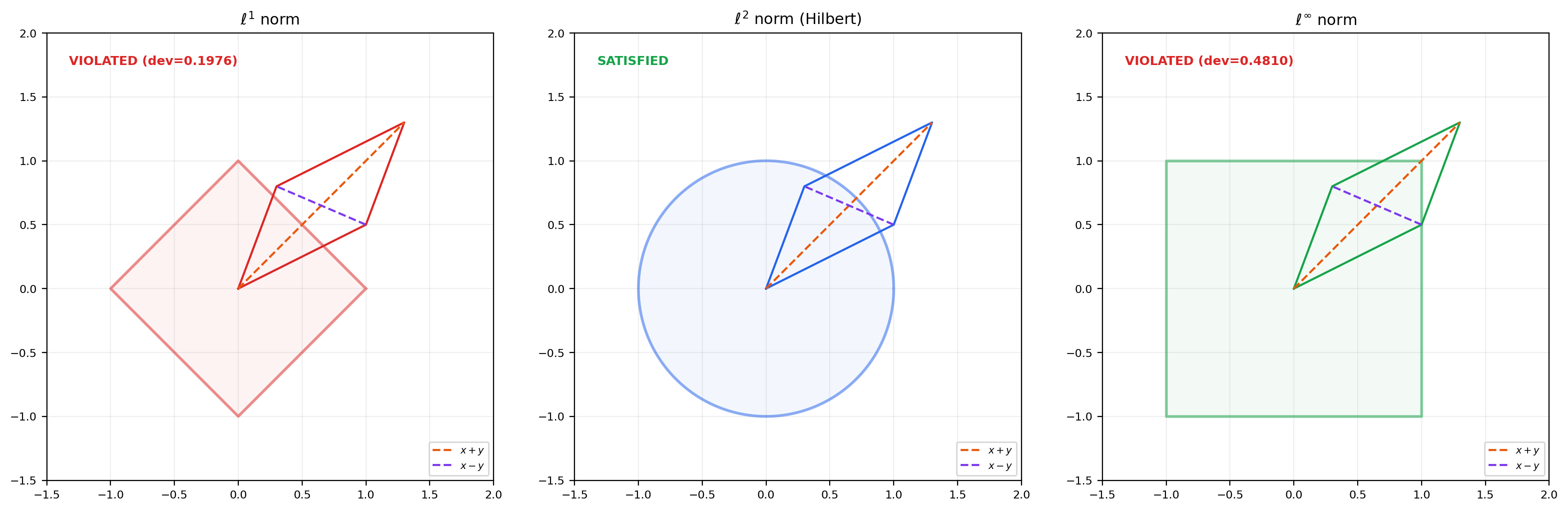
💡 Remark 2 (The Parallelogram Law Characterizes Inner Product Norms)
The parallelogram law is not just a consequence of inner products — it characterizes them. A normed space has a norm induced by an inner product if and only if the parallelogram law holds. When it does, the polarization identity recovers the inner product from the norm:
This is why for is a Banach space but not a Hilbert space: the and norms violate the parallelogram law. The norm is the only norm that comes from an inner product.
4. Hilbert Spaces
📐 Definition 2 (Hilbert Space)
A Hilbert space is a complete inner product space — an inner product space in which every Cauchy sequence converges (in the norm induced by the inner product).
Equivalently: is a Banach space whose norm satisfies the parallelogram law.
📝 Example 5 (Catalog of Hilbert Spaces)
The following are Hilbert spaces (complete inner product spaces):
- with the standard inner product — finite-dimensional, hence automatically complete.
- with — completeness is the Riesz-Fischer theorem (Topic 27, Theorem 5) for counting measure.
- with — completeness is Riesz-Fischer for a general measure.
- — the Hilbert space where Fourier analysis lives (Topic 22).
The following are inner product spaces that are not Hilbert spaces (not complete):
- with — not complete under this inner product because Cauchy sequences of continuous functions can converge to discontinuous functions.
- The space of polynomials on with the inner product — not complete because polynomials are dense in but do not exhaust it.
💡 Remark 3 (Why Hilbert Spaces Are Special)
Every Hilbert space is a Banach space. The converse is emphatically false: , , with the sup-norm, and for are all Banach but not Hilbert — their norms violate the parallelogram law. The distinction matters because the inner product gives us orthogonality, and orthogonality gives us the projection theorem (Theorem 4), which has no analog in general Banach spaces. The Baire-powered theorems from Topic 30 (Uniform Boundedness, Open Mapping, Closed Graph) still apply — a Hilbert space is a Banach space, so all Banach-space theorems carry over — but the inner product adds an entire geometric toolkit on top.
5. Orthogonality
📐 Definition 3 (Orthogonality and Orthogonal Complement)
Two vectors are orthogonal (written ) if .
For a subset , the orthogonal complement is:
is always a closed subspace of , regardless of whether itself is a subspace.
The Pythagorean theorem extends to inner product spaces: if , then . This is the geometric identity that the projection theorem exploits.
🔷 Theorem 3 (Orthogonal Decomposition)
Let be a closed subspace of a Hilbert space . Then every can be written uniquely as:
where and . In other words, (orthogonal direct sum), and .
This is one of the most powerful structural results in functional analysis. It says that a closed subspace of a Hilbert space has a complement — and not just any complement, but an orthogonal one. In general Banach spaces, closed subspaces need not have complements at all.
📝 Example 6 (Orthogonal Complement in ℝ³)
In with the standard inner product, let be the -plane: . Then — the -axis. Every vector decomposes uniquely into its and components.
📝 Example 7 (Orthogonal Complement in L²)
In , let (even functions). Then (odd functions). Every function decomposes uniquely as where and .
6. The Projection Theorem
This is the central result of the topic. The projection theorem says: in a Hilbert space, every point has a unique closest point in any closed convex subset — and when the subset is a subspace, the closest point is the orthogonal projection.
🔷 Theorem 4 (Projection Theorem)
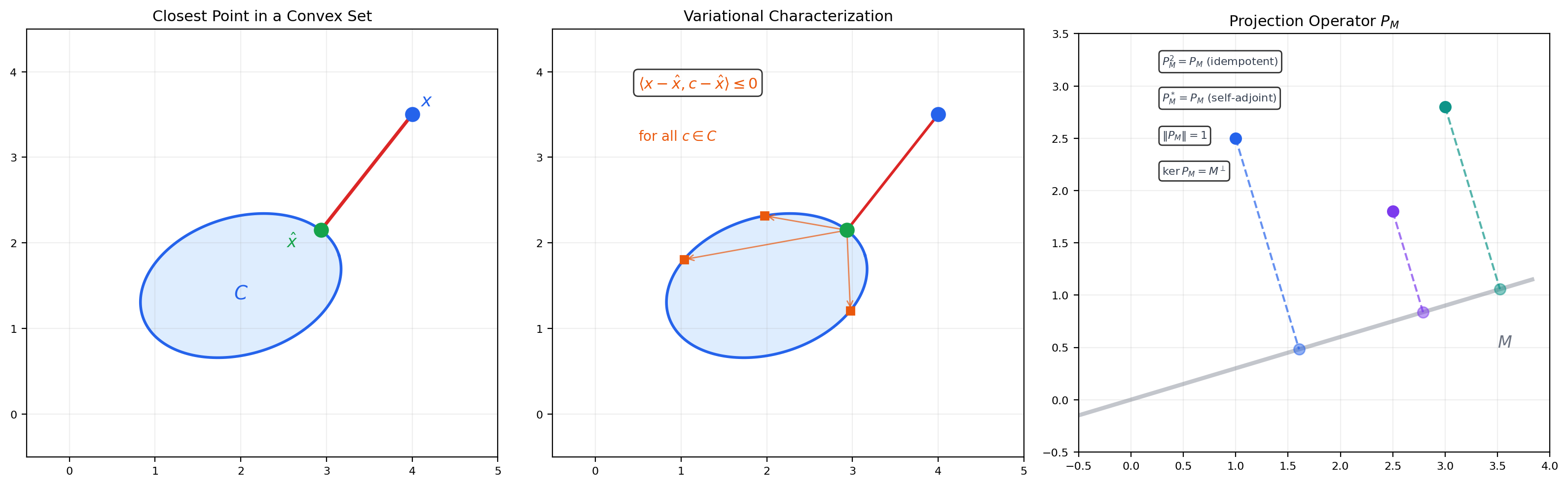
Let be a Hilbert space and a nonempty, closed, convex subset. For every , there exists a unique such that:
When is a closed subspace, the minimizer is characterized by the orthogonality condition: for all .
Proof.
We prove existence, uniqueness, and the orthogonality characterization.
Step 1. Setup. Let . Choose a minimizing sequence with .
Step 2. The minimizing sequence is Cauchy. Apply the parallelogram law to and :
The left side involves and . Since is convex, , so , which gives . Thus:
Since and , the right side . So is Cauchy.
Step 3. Existence. Since is complete and is closed, the Cauchy sequence converges to some . Continuity of the norm gives .
Step 4. Uniqueness. If both achieve the minimum , apply the parallelogram law to and :
So .
Step 5. Orthogonality (when is a subspace). Suppose is the closest point to . For any and , , so:
This gives for all . Taking (assuming ) gives , hence .
The parallelogram law is essential in Step 2. In a Banach space without an inner product (where the parallelogram law fails), the closest point may not exist or may not be unique. This is the fundamental reason Hilbert spaces are geometrically better behaved than general Banach spaces.
📐 Definition 4 (Orthogonal Projection Operator)
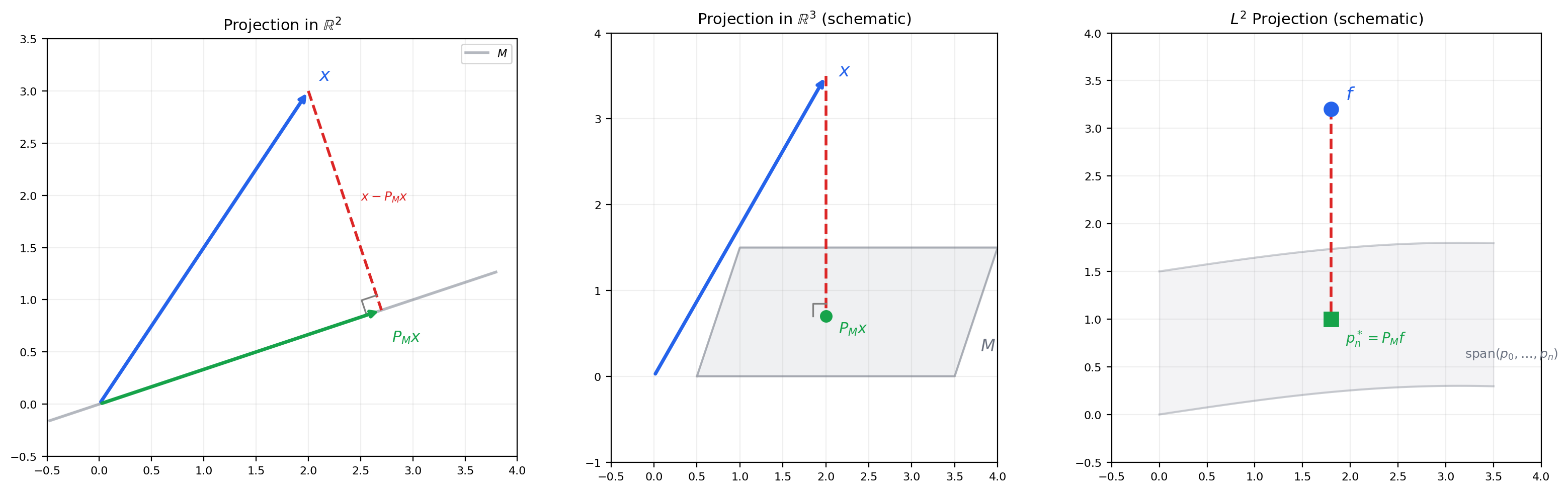
Let be a closed subspace of a Hilbert space . The orthogonal projection maps each to its unique closest point . It satisfies:
- is linear and bounded with (unless ).
- (idempotent: projecting twice is the same as projecting once).
- (self-adjoint: ).
- and .
- .
📝 Example 8 (Projection in ℝⁿ)
In , if is the span of an orthonormal set , then:
The residual is (where extends to an ONB of ). The Pythagorean theorem gives .
📝 Example 9 (Best L² Approximation as Projection)
Finding the best approximation to a function by polynomials of degree is exactly orthogonal projection onto the -dimensional subspace . The error is orthogonal to every polynomial of degree . When we use the Legendre polynomials as an orthonormal basis for on , the projection formula becomes:
This is best approximation in the sense, developed abstractly in Topic 20 and now revealed as a special case of the projection theorem.
The projection PMx is the closest point in M to x. The residual x − PMx is perpendicular to M — this is the geometric content of the projection theorem.
7. Orthonormal Bases
📐 Definition 5 (Orthonormal System and Orthonormal Basis)
An orthonormal system (ONS) in is a set such that (each vector has unit norm and distinct vectors are orthogonal).
An orthonormal basis (ONB) is a maximal orthonormal system — equivalently, an ONS such that (the closed linear span is all of ).
An ONB is not a Hamel basis (which requires every vector to be a finite linear combination). An ONB allows infinite linear combinations — series that converge in the norm.
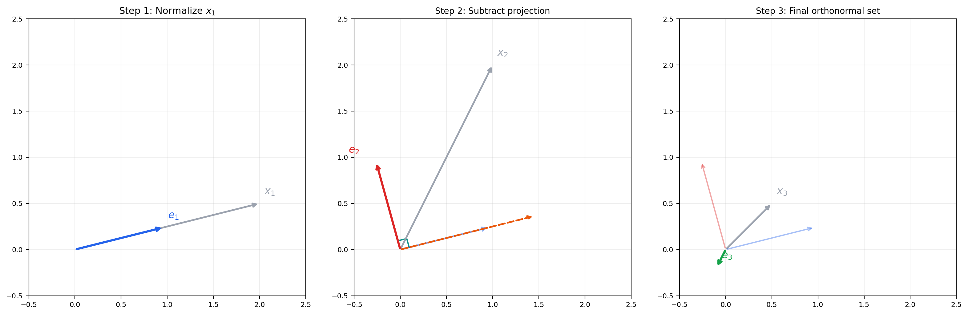
🔷 Theorem 5 (Gram-Schmidt Orthonormalization)
Given a finite or countably infinite linearly independent set in an inner product space, the Gram-Schmidt process produces an orthonormal set with the property that for every .
The algorithm: set , . For :
Each is obtained by subtracting the projection of onto the span of . What remains is the component of orthogonal to the previous basis vectors.
Input vectors shown. Press Next to begin orthonormalization.
Gram-Schmidt subtracts the projection of each new vector onto the already-orthonormalized set, then normalizes. Orange dashed lines show the projections being removed.
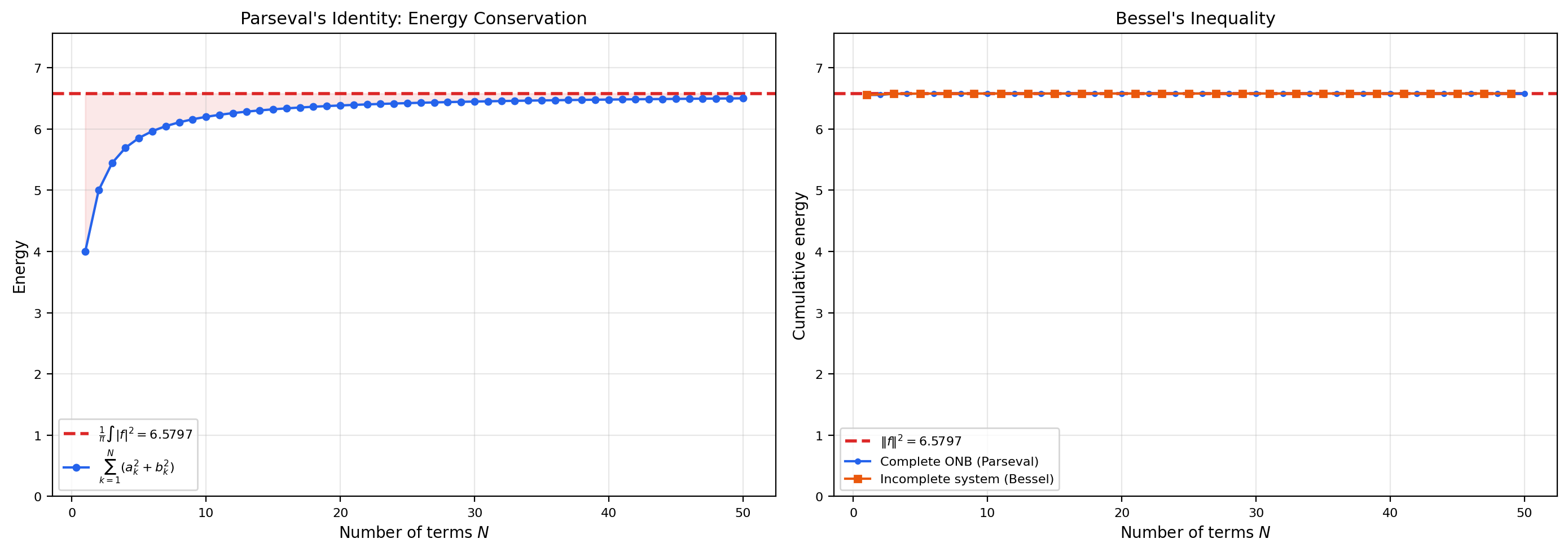
🔷 Theorem 6 (Bessel's Inequality)
Let be an orthonormal system in a Hilbert space . For every :
The coefficients are called the Fourier coefficients of with respect to the ONS.
Proof.
For any finite , let be the projection of onto . By orthogonality of the residual:
Now (because the are orthonormal). So:
This holds for every , so the series converges and is bounded by .
🔷 Theorem 7 (Parseval's Identity)
Let be an orthonormal basis for a Hilbert space . Then for every :
Equivalently, (convergence in norm).
Proof.
Bessel’s inequality gives . For the reverse, since is an ONB, the closed span of is all of . So for every , there exists and scalars with .
The projection minimizes the distance from to (by the projection theorem), so .
Therefore , and since is arbitrary, .
Parseval’s identity is a conservation law: it says the “energy” of is fully captured by its Fourier coefficients. For with the trigonometric ONB, Parseval becomes — the concrete version from Topic 22.
🔷 Proposition 1 (Separable Hilbert Spaces Have Countable ONBs)
A Hilbert space is separable (has a countable dense subset) if and only if it admits a countable orthonormal basis. Every separable infinite-dimensional Hilbert space is isometrically isomorphic to .
📝 Example 10 (Fourier Basis as an Orthonormal Basis)
The trigonometric system is an orthonormal basis for . Parseval’s identity in this basis is the classical result that the Fourier coefficients capture all the energy of the function. This concrete Fourier theory from Topic 22 is a special case of the abstract Hilbert space theory developed here.
💡 Remark 4 (All Separable Hilbert Spaces Are the Same)
Proposition 1 says something remarkable: up to isometric isomorphism, there is only one separable infinite-dimensional Hilbert space — . Whether you work with , (with respect to a finite measure), or any other separable Hilbert space, the abstract structure is the same. The isomorphism maps any ONB to the standard basis of . This universality is unique to Hilbert spaces — for Banach spaces, and are genuinely different spaces when .
8. The Riesz Representation Theorem
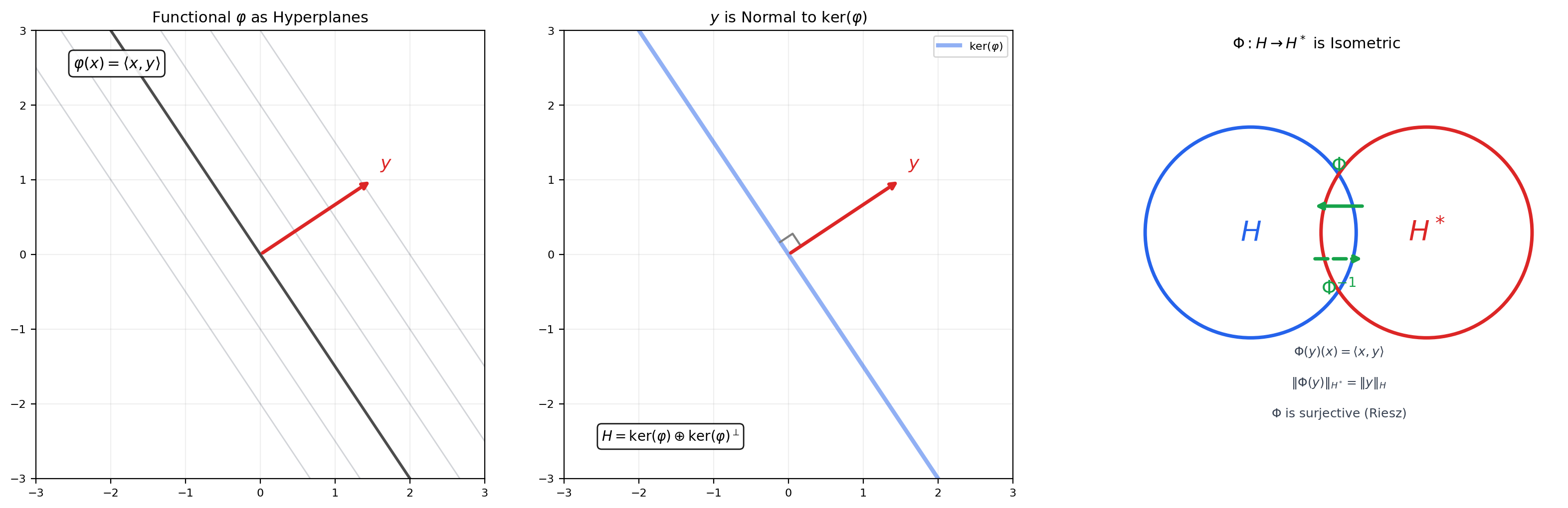
The Riesz representation theorem is the most important structural result about Hilbert spaces. It says that the dual space (all bounded linear functionals on ) is isometrically isomorphic to itself — every bounded linear functional is “represented” by a unique vector via the inner product.
🔷 Theorem 8 (Riesz Representation Theorem)
Let be a Hilbert space and a bounded linear functional. Then there exists a unique such that:
Moreover, . The map is a linear isometric isomorphism (in the real case; conjugate-linear in the complex case).
Proof.
Step 1. The kernel of . If , take . Assume . The kernel is a closed subspace of (closed because is continuous).
Step 2. The codimension-1 decomposition. Since , . By the orthogonal decomposition theorem (Theorem 3), . Since is a nonzero functional, — pick any with .
Step 3. Construct the representing vector. Set (in the real case, ). For any , write where and .
Then:
Step 4. Uniqueness. If for all , then for all . Taking gives , so .
Step 5. Isometry. by Cauchy-Schwarz, with equality achieved at .
💡 Remark 5 (Contrast with Banach-Space Duality)
In Topic 30, computing the dual space required the full Hahn-Banach machinery, and the dual of required the Radon-Nikodym theorem (Topic 28). For Hilbert spaces, the Riesz representation theorem replaces all of this with a single, geometric argument based on the projection theorem. The dual of is itself — there is no separate “dual space” to worry about. This is why optimization in Hilbert spaces (gradient descent, proximal methods) is fundamentally simpler than in general Banach spaces (mirror descent, Fenchel conjugates) — the gradient is a vector in the same space, not an element of a dual space that needs to be mapped back.
🔷 Corollary 1 (Hilbert Spaces Are Reflexive)
Every Hilbert space is reflexive: the canonical embedding is surjective. This follows immediately from the Riesz representation theorem applied twice: and .
Reflexivity was an open question for general Banach spaces in Topic 30 (Remark 7). For Hilbert spaces, it is an immediate corollary.
9. Compact Operators and the Spectral Theorem
📐 Definition 6 (Compact Operator)
A bounded linear operator is compact if it maps every bounded set to a relatively compact set (a set whose closure is compact). Equivalently, maps bounded sequences to sequences with convergent subsequences.
Compact operators are the “almost finite-dimensional” operators. They can be approximated by finite-rank operators. In finite dimensions, every linear operator is compact.
📐 Definition 7 (Self-Adjoint Operator)
A bounded linear operator is self-adjoint (or symmetric) if:
Self-adjoint operators are the infinite-dimensional generalization of symmetric matrices. Their eigenvalues are real, and eigenvectors for distinct eigenvalues are orthogonal — exactly as in the finite-dimensional spectral theorem.
🔷 Theorem 9 (Spectral Theorem for Compact Self-Adjoint Operators)
Let be a compact self-adjoint operator on a Hilbert space . Then:
- The eigenvalues of are real, and form a sequence converging to (or are finitely many).
- Eigenvectors corresponding to distinct eigenvalues are orthogonal.
- , where are the eigenspaces.
- For every :
where is an orthonormal basis of eigenvectors for , with .
Proof.
Step 1. Eigenvalues are real. If with , then , so .
Step 2. Eigenvectors for distinct eigenvalues are orthogonal. If and with , then , so , giving .
Step 3. The first eigenvalue exists via the Rayleigh quotient. Define (which equals the operator norm for self-adjoint ). There exists a sequence on the unit sphere with . By compactness, has a convergent subsequence. One shows the subsequence of converges to an eigenvector with eigenvalue .
Step 4. Induction on orthogonal complements. The subspace is invariant under (because is self-adjoint). Restrict to — the restriction is still compact and self-adjoint — and apply Step 3 to find . Continue inductively.
Step 5. Eigenvalues converge to 0. If the eigenvalues do not converge to 0, there exists and a subsequence with . The eigenvectors are orthonormal, so — the sequence has no convergent subsequence, contradicting compactness of .
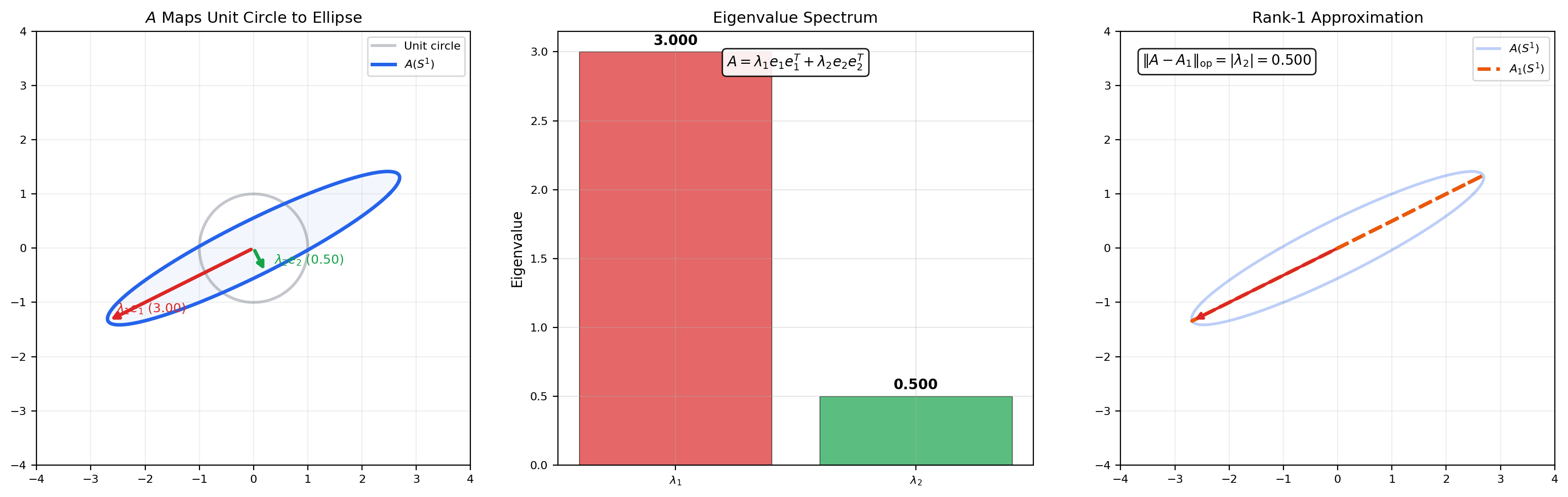
📝 Example 11 (Spectral Decomposition of a Symmetric Matrix)
A symmetric matrix has eigenvalues with orthogonal eigenvectors. The spectral decomposition is . The unit circle maps to an ellipse with semi-axes and along the eigenvector directions. The rank-1 approximation is the best rank-1 approximation in the operator norm (Eckart-Young theorem) — this is PCA in finite dimensions.
A symmetric matrix maps the unit circle to an ellipse whose axes are the eigenvectors, scaled by eigenvalues. The rank-1 approximation λ₁v₁v₁ᵀ keeps only the dominant eigendirection.
💡 Remark 6 (Beyond Compact Self-Adjoint)
The spectral theorem for compact self-adjoint operators is a stepping stone to the general spectral theorem for bounded (or unbounded) self-adjoint operators, which replaces the discrete eigenvalue sum with a spectral integral over a projection-valued measure. This general version — due to von Neumann — is essential for quantum mechanics (where observables are self-adjoint operators) but is beyond the scope of this topic. We note only that our compact case captures the most common finite-dimensional intuition: diagonalization with orthogonal eigenvectors.
10. Reproducing Kernel Hilbert Spaces
This section is the strongest bridge between Hilbert space theory and machine learning. A reproducing kernel Hilbert space (RKHS) is a Hilbert space of functions in which “evaluate the function at a point” is a continuous operation — and by the Riesz representation theorem, evaluation at each point is an inner product with a special element.
📐 Definition 8 (Reproducing Kernel Hilbert Space)
A reproducing kernel Hilbert space (RKHS) is a Hilbert space of functions such that for every , the evaluation functional is a bounded linear functional on .
By the Riesz representation theorem (Theorem 8), there exists a unique such that for all . The function defined by is called the reproducing kernel of .
🔷 Theorem 10 (The Reproducing Property)
Let be an RKHS with kernel . Then for every and every :
This is the reproducing property: evaluating at is the same as taking the inner product of with the kernel function .
🔷 Theorem 11 (Moore-Aronszajn Theorem)
For every positive-definite kernel (meaning for all finite sets of points and coefficients), there exists a unique RKHS with as its reproducing kernel.
Proof sketch. Start with the pre-Hilbert space of finite linear combinations with inner product . Positive-definiteness of ensures this inner product is well-defined and positive. Complete the space to get .
📝 Example 12 (Common Kernels and Their RKHS)
- Linear kernel: . The RKHS is the space of linear functions.
- Polynomial kernel (degree ): . The RKHS consists of polynomials of degree .
- Gaussian (RBF) kernel: . The RKHS is an infinite-dimensional space of smooth functions that is dense in — this kernel is universal.
🔷 Theorem 12 (Representer Theorem)
Let be an RKHS with kernel , and let be training data. The minimizer of the regularized empirical risk:
(where is any loss function and ) lies in the finite-dimensional subspace spanned by the kernel evaluations at training points:
for some coefficients .
Proof.
Decompose where and for all (using the projection theorem).
By the reproducing property, .
So the loss depends only on . Meanwhile, . Therefore setting does not increase the loss and strictly decreases the regularization unless already. The minimizer has , hence .
The representer theorem is the mathematical foundation of kernel methods in machine learning. It says that even though may be infinite-dimensional (as for the Gaussian kernel), the optimal function lives in a finite-dimensional subspace whose dimension is the number of training points — not the dimension of .
💡 Remark 7 (Why the Representer Theorem Matters for ML)
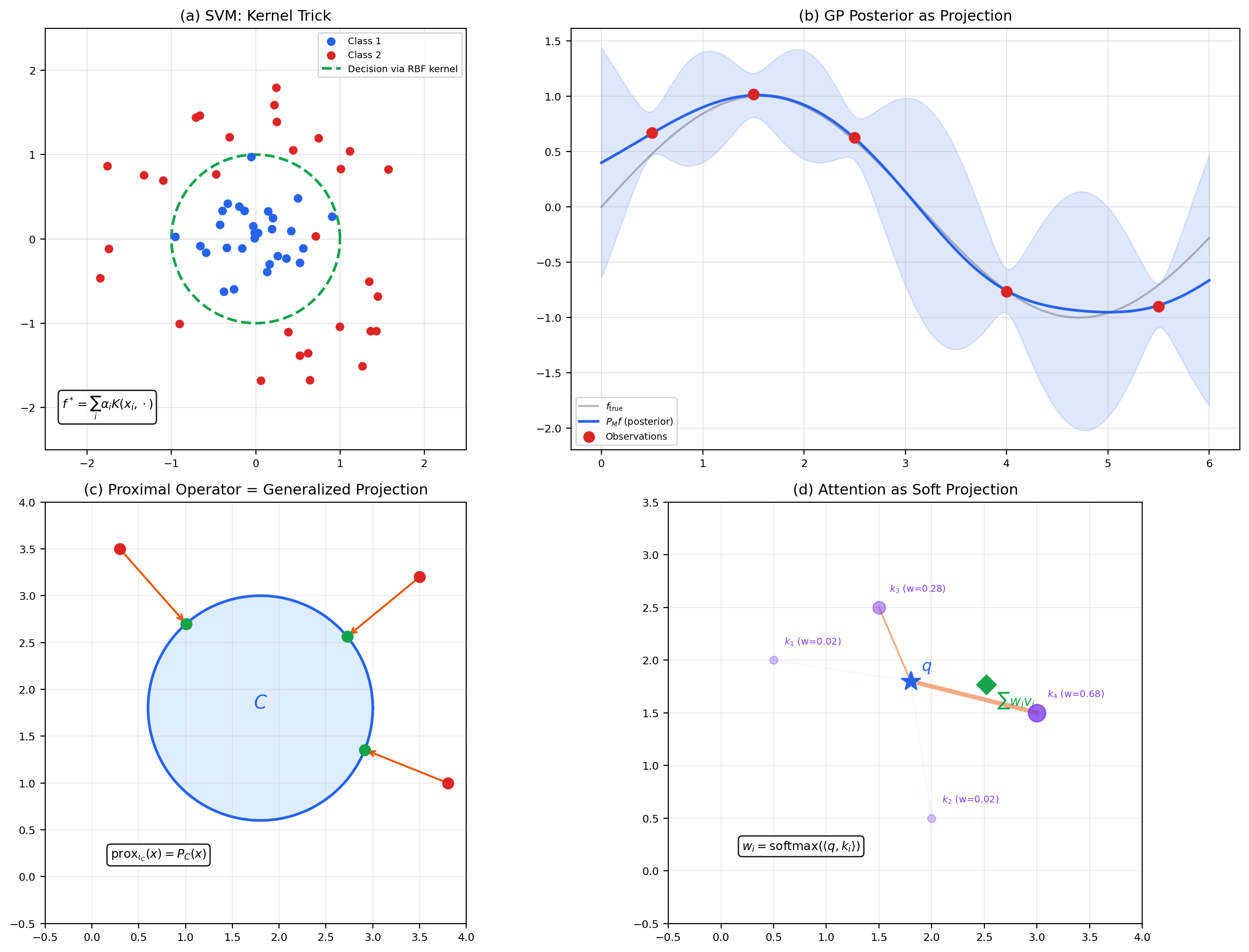
The representer theorem turns an infinite-dimensional optimization problem into a finite-dimensional one. Instead of searching over all functions in , we search over coefficients . The kernel trick then allows us to compute everything — predictions, regularization, gradients — using only kernel evaluations , without ever constructing the (possibly infinite-dimensional) feature map explicitly. This is why SVMs, Gaussian processes, and kernel PCA scale with the number of training points rather than the dimension of the feature space. See Kernel Methods on formalML for the full development.
Click in the right panel to add training points (up to 8). Click near an existing point to remove it. The representer theorem guarantees f* lives in the span of kernel evaluations at training points.
11. Connections to Statistics
Hilbert-space geometry — projections, orthogonality, RKHS — is the natural language of regression, kernel methods, and Gaussian processes.
OLS as orthogonal projection
OLS is the orthogonal projection of onto in as a Hilbert space. The Pythagorean decomposition underlies the ANOVA identity . The normal equations express the orthogonality of residuals to the column space. See formalStatistics Linear Regression.
Kernel methods and KDE
Mercer’s theorem expresses positive-definite kernels as inner products in a feature Hilbert space. The reproducing property in an RKHS is the kernel-methods workhorse. Gaussian-process and RKHS methods for smoothing are Hilbert-space regression. See formalStatistics Kernel Density Estimation.
Gaussian-process priors
GP priors over functions are specified by a mean and covariance kernel — a Hilbert-space structure. The Cameron–Martin space associated with a GP prior is the RKHS of the kernel; posterior contractions happen in this Hilbert-space geometry. See formalStatistics Bayesian Foundations & Prior Selection.
12. Connections to ML
📝 Example 13 (Kernel Methods and SVMs)
Support vector machines solve a classification problem by finding a maximum-margin hyperplane in an RKHS. The SVM dual problem involves only kernel evaluations — the representer theorem guarantees the optimal classifier is , where the are the Lagrange multipliers (support vector coefficients). See Kernel Methods on formalML.
📝 Example 14 (Gaussian Processes as Projections in RKHS)
A Gaussian process (GP) prior on functions induces an RKHS. The GP posterior mean at a test point , given training data, is the orthogonal projection of onto the subspace . The posterior variance measures the squared distance from to this subspace — it is where . See Generative Modeling on formalML.
📝 Example 15 (Proximal Operators as Projections)
The proximal operator is a generalization of orthogonal projection. When is the indicator function of a closed convex set , — exactly the projection from Theorem 4. Proximal gradient descent, ISTA/FISTA, and ADMM all use projections in Hilbert spaces as their core operations. See Optimization Theory on formalML.
📝 Example 16 (Attention as Projection)
In the transformer attention mechanism, the output for a query is — a weighted combination of values , where the weights are inner-product similarities between the query and keys. This is a “soft projection” of onto the subspace spanned by keys, with the inner product determining the projection weights. Standard orthogonal projection is the “hard” limit as the softmax temperature goes to zero.
13. Computational Notes
All of the algorithms in this topic have efficient numerical implementations.
Inner products and norms. In NumPy: np.dot(x, y) or x @ y for the Euclidean inner product, np.linalg.norm(x) for the norm. For weighted inner products: np.dot(w * x, y).
Projection. Onto a subspace with orthonormal basis (columns are ONB vectors): P = E @ E.T, then proj = P @ x. For a general basis, Gram-Schmidt first or use the normal equations: proj = E @ np.linalg.solve(E.T @ E, E.T @ x).
Gram-Schmidt. NumPy: np.linalg.qr(V) computes the QR decomposition, where contains the orthonormalized vectors. For step-by-step visualization, implement the loop explicitly as in the notebook.
Kernel methods. Build the Gram matrix , solve alpha = np.linalg.solve(K + lambda * I, y), predict via f_star = K_test @ alpha.
Eigendecomposition. For a symmetric matrix: eigenvalues, eigenvectors = np.linalg.eigh(A). Use eigh (not eig) for symmetric matrices — it guarantees real eigenvalues and orthogonal eigenvectors.
14. Summary
| Concept | Key Result | Why It Matters |
|---|---|---|
| Inner product | Adds angles and orthogonality to normed spaces | Enables the geometric toolkit that norms lack |
| Cauchy-Schwarz | Makes angles well-defined; controls all inner-product estimates | |
| Parallelogram law | Characterizes inner product norms; essential in projection proof | |
| Hilbert space | Complete inner product space | The “good” geometric spaces where all theorems work |
| Projection theorem | Unique closest point in closed convex sets | The foundation for everything below |
| Orthonormal bases | Parseval’s identity: | Generalized Fourier analysis; every separable Hilbert space ≅ ℓ² |
| Riesz representation | via | Collapses dual-space complexity; Hilbert spaces are self-dual |
| Spectral theorem | Compact self-adjoint | Eigendecomposition with orthogonal eigenvectors; foundation of PCA |
| RKHS | Evaluation via inner product; representer theorem for kernel methods |
15. Looking Ahead
The next and final topic in Track 8 is Calculus of Variations — the study of functionals defined on function spaces, and the search for functions that minimize (or maximize) them. The Euler-Lagrange equation, the direct method for existence of minimizers, and weak solutions to PDEs all rely on the Hilbert space infrastructure we have built here. The projection theorem provides existence of minimizers in reflexive spaces; the Riesz representation theorem turns the weak formulation of PDEs into a Hilbert-space problem; and Sobolev spaces — the natural domains for variational problems — are Hilbert spaces when .
Where this topic added one axiom (the inner product) to Banach spaces and gained geometric power, Topic 32 adds one more idea — variation — to function spaces and gains the ability to find optimal functions. The staircase of abstraction reaches its summit.
Connections & Further Reading
Prerequisites — topics you need first
Normed & Banach Spaces
Every Hilbert space is a Banach space. Topic 30 provides normed spaces, completeness, bounded operators, and dual spaces — Topic 31 adds the inner product that makes all of these dramatically simpler.
Lp Spaces
L^2 is the canonical Hilbert space — the inner product generalizes the L^2 norm from Topic 27. Bessel's inequality and Parseval's identity generalize the concrete L^2 orthogonality from Fourier series.
Fourier Series & Orthogonal Expansions
Fourier analysis on L^2[-π,π] is the concrete instance of the abstract Hilbert space theory developed here — trigonometric functions as an orthonormal basis, Parseval's identity as energy conservation.
Approximation Theory
Best L^2 approximation is orthogonal projection onto a finite-dimensional subspace. Legendre polynomials and Chebyshev polynomials are orthonormal bases for specific weighted L^2 spaces.
Radon-Nikodym & Probability Densities
Conditional expectation is the orthogonal projection of an L^2 random variable onto a sub-σ-algebra. The projection theorem provides the existence and uniqueness.
Metric Spaces & Topology
Topic 29 built the metric foundation (completeness, compactness). Topic 31 adds inner-product structure on top of the normed (Topic 30) and metric (Topic 29) layers.
Where this leads — next in formalCalculus
On to formalStatistics — where this calculus powers inference
Linear Regression
OLS is the orthogonal projection of y onto col(X) in ℝⁿ as Hilbert space. The Pythagorean decomposition ‖y‖² = ‖ŷ‖² + ‖y - ŷ‖² underlies the ANOVA identity SST = SSR + SSE. The normal equations XᵀXβ̂ = Xᵀy express the orthogonality of residuals to the column space.
Kernel Density Estimation
Mercer's theorem expresses positive-definite kernels as inner products in a feature Hilbert space. The reproducing property ⟨K(·,x), f⟩ = f(x) in an RKHS is the kernel-methods workhorse. Gaussian-process and RKHS methods for smoothing are Hilbert-space regression.
Bayesian Foundations And Prior Selection
Gaussian-process priors over functions are specified by a mean and covariance kernel — a Hilbert-space structure. The Cameron–Martin space associated with a GP prior is the RKHS of the kernel; posterior contractions happen in this Hilbert-space geometry.
On to formalML — where this calculus powers ML
Gradient Descent
Proximal operators are defined via orthogonal projections in Hilbert spaces. The Riesz identification lets us interpret gradients as descent directions in dual coordinates, and Hilbert-space gradient descent converges because Riesz turns dual-space gradients into primal-space descent directions — no separate dual-space bookkeeping needed.
Semiparametric Inference
§2's $L^2(P)$-based geometry — tangent spaces as closed subspaces, orthogonal complements via the inner product, the projection theorem for the EIF — is a direct application of Hilbert-space theory. The §3 Riesz representation theorem and §4 Pythagorean lower bound both live entirely in the Hilbert-space picture.
References
- book Kreyszig (1978). Introductory Functional Analysis with Applications Chapters 3–4 (inner product spaces, Hilbert spaces). Comprehensive and accessible.
- book Conway (1990). Functional Analysis Chapters 1–2 (Hilbert spaces, projection, Riesz). Clean modern treatment.
- book Brezis (2011). Functional Analysis, Sobolev Spaces and Partial Differential Equations Chapter 5 (Hilbert spaces). Concise proofs with applications.
- book Folland (1999). Real Analysis: Modern Techniques and Their Applications Chapter 5 (elements of functional analysis). Rigorous with measure-theoretic context.
- book Schölkopf & Smola (2002). Learning with Kernels RKHS theory for machine learning. The representer theorem and kernel trick.