Radon-Nikodym & Probability Densities
Turning measures into functions — from the Radon-Nikodym theorem through conditional expectation and change of measure to the rigorous foundations of probability densities, importance sampling, and Bayesian inference.
Abstract. Every probability density function you have ever written down — every Gaussian bell curve, every softmax output, every generative model's learned distribution — is a Radon-Nikodym derivative. The Radon-Nikodym theorem is the single theorem that turns measure theory into probability theory: it says that when one measure is absolutely continuous with respect to another, the relationship can be captured by a single integrable function. We prove this using the L² projection machinery from Topic 27, reducing the existence of densities to a Hilbert-space projection argument. The theorem's reach is extraordinary: probability densities are Radon-Nikodym derivatives with respect to Lebesgue measure. Conditional expectation — the engine behind regression, Bayesian inference, and reinforcement learning — is a Radon-Nikodym derivative with respect to a sub-sigma-algebra. Importance sampling weights are Radon-Nikodym derivatives between proposal and target measures. KL divergence is the expected log-Radon-Nikodym derivative. This topic completes the Measure and Integration track by bridging the gap between abstract measure theory and the concrete probabilistic tools that machine learning practitioners use every day.
1. Three Puzzles the Radon-Nikodym Theorem Solves
Topic 27 organized integrable functions into the spaces — vector spaces with a norm, a notion of distance, and (for ) an inner product and an orthogonal-projection theorem. Along the way we used the Radon-Nikodym theorem as a black box twice: once in Section 9, when we previewed projection, and once in Section 10, when we proved duality and said “by the Radon-Nikodym theorem (which we will prove in Topic 28; for now we use it as a black box), absolute continuity implies that has a density…”. This topic pays the debt. The von Neumann proof uses the projection theorem from Topic 27 §9 — the same tool we previewed for regression — to reduce the existence of densities to a single Hilbert-space projection argument.
The pivot in this topic is from spaces of functions to measures as functions. Topic 27 asked “how do we organize integrable functions?”; Topic 28 asks “when can one measure be represented as a function against another?” The answer makes measure theory into probability theory. Three concrete questions motivate the theorem.
1. What exactly is a “probability density”? Every ML practitioner writes and calls it “the density of the standard normal.” But a probability measure assigns numbers to sets, not points — and when is continuous, for every individual . So what is ? It is not . The Radon-Nikodym theorem answers: is the derivative of the probability measure with respect to Lebesgue measure — a function whose integral recovers . The “density” is a derivative in a precise measure-theoretic sense, not a metaphor.
2. What is , really? Introductory courses define conditional expectation by “averaging over the slice where .” But when is continuous, the event has probability zero — you cannot condition on a zero-probability event without doing some work first. Measure-theoretic conditional expectation resolves this: is the Radon-Nikodym derivative of a certain restricted measure, and (when ) it is the best predictor of given . Regression algorithms — linear regression, random forests, neural networks — are all approximating this single object.
3. How do importance-sampling weights work? To estimate using samples from a different distribution , we reweight: where . But what is ? It is a Radon-Nikodym derivative — the function that converts integration with respect to into integration with respect to . The reweighting identity is a change-of-measure formula, and its validity requires (every -null set is -null). When importance sampling fails — when the variance of the weights blows up — it is almost always because the absolute-continuity hypothesis is silently violated in some region of the sample space.
These three questions are the same question from three angles: when can a measure be written as a function against another measure, and what is that function? The answer is the Radon-Nikodym derivative, and the theorem that produces it is the bridge from measure theory to probability theory.
2. Absolute Continuity and Mutual Singularity
Before stating the theorem we need two definitions. Both describe relationships between measures, and the contrast between them is sharp: absolutely continuous measures share their null sets; mutually singular measures live on disjoint sets.
📐 Definition 1 (Absolute continuity of measures)
Let and be measures on a measurable space . We say is absolutely continuous with respect to , written , if for every ,
In words: every -null set is also a -null set. The relationship is one-directional — does not imply .
📐 Definition 2 (Mutual singularity)
Two measures and on are mutually singular, written , if there exist disjoint sets with such that
In words: the two measures live on disjoint pieces of — assigns all its mass to , and assigns all its mass to . They cannot see each other.
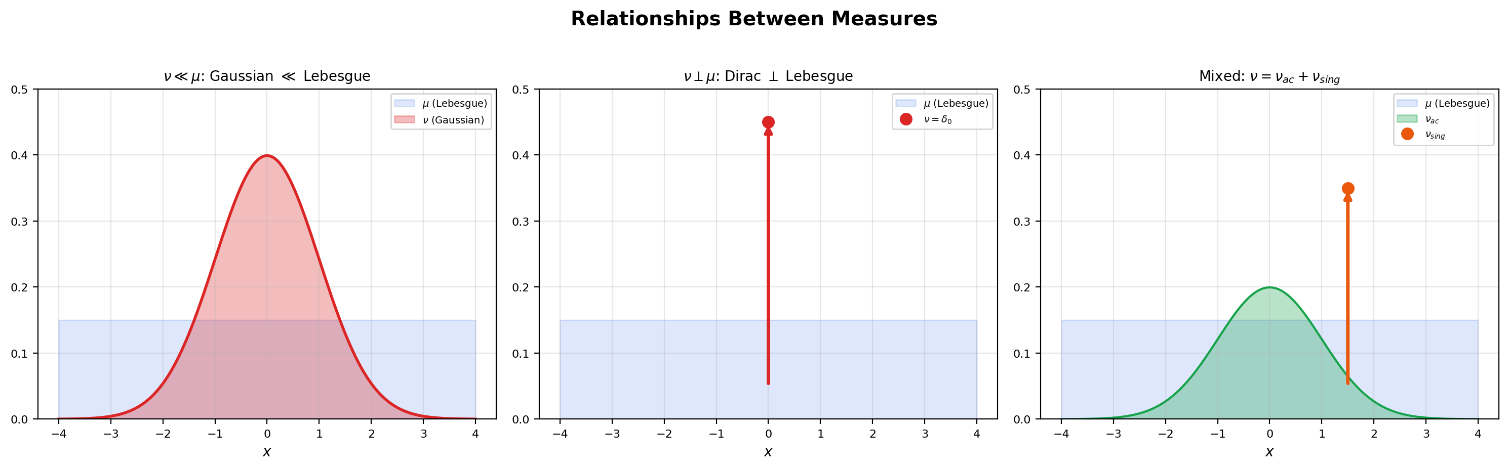
📝 Example 1 (Gaussian measure is absolutely continuous w.r.t. Lebesgue)
Let be the standard normal probability measure on and let denote Lebesgue measure. If — say, is a countable set or a Cantor-type set of Lebesgue measure zero — then
because the Lebesgue integral over a null set is always zero. So . The density is — as we will see in Section 3 — the Radon-Nikodym derivative . Every Gaussian distribution you have ever computed with is a worked example of absolute continuity.
📝 Example 2 (Dirac measure is singular w.r.t. Lebesgue)
Let be the Dirac measure at : if , else . Then . To verify, take and . Then (a single point has Lebesgue measure zero) and (the Dirac mass is not at any point of ). The two measures partition into the single point where lives and the rest of the line where lives. They cannot be combined into a density relationship — there is no function with , because integrating any Lebesgue-integrable function over gives zero.
📝 Example 3 (Counting measure on $\mathbb{Z}$ is singular w.r.t. Lebesgue on $\mathbb{R}$)
Let be counting measure on that assigns measure to each integer and to non-integers; equivalently, . Then . Take and . Then (a countable set has Lebesgue measure zero) and (no integers in ). Discrete and continuous measures live on disjoint supports. This is why you cannot write a Poisson distribution as — the Poisson measure is supported on , which is a -null set.
💡 Remark 1 (Absolute continuity of measures vs. absolute continuity of functions)
The reader may know “absolutely continuous function” from calculus — a function is absolutely continuous if for every there is a such that any finite collection of disjoint subintervals with total length less than produces total variation less than . These two concepts are related but distinct: a function is absolutely continuous on if and only if there exists with , and equivalently the signed measure is absolutely continuous (in our measure-theoretic sense) with respect to Lebesgue measure. The function-theoretic notion is a special case of the measure-theoretic one.
💡 Remark 2 ($\sigma$-finiteness is essential)
The Radon-Nikodym theorem requires both and to be -finite: is a countable union of measurable sets of finite measure under each. Without this, the theorem can fail. The standard counterexample is counting measure on (which is not -finite — the only set of finite counting measure is a finite set, and is not a countable union of finite sets) compared with Lebesgue measure: holds vacuously (the only -null set is ), but no integrable density can exist because and disagree on every uncountable measurable set. In probability applications, -finiteness is automatic: every probability measure is finite (hence -finite), so this hypothesis is rarely something the practitioner needs to check.
3. The Radon-Nikodym Derivative
We can now define the central object of the topic. The definition is short — it just names a function that satisfies a particular integral identity — and the substance of the topic is showing that such a function actually exists whenever absolute continuity holds.
📐 Definition 3 (The Radon-Nikodym derivative)
Let and be -finite measures on with . If there exists a non-negative measurable function such that
then is called the Radon-Nikodym derivative of with respect to , written
The notation is deliberately Leibniz-style: behaves like a derivative in several senses (chain rule, inverse rule), as we will see in Section 5.
🔷 Proposition 1 (Uniqueness of the R-N derivative ($\mu$-a.e.))
If and are both Radon-Nikodym derivatives of with respect to , then -almost everywhere.
Proof.
Suppose for every measurable , so
Let . Then on , and forces (an integral of a strictly positive function over a set is zero only when the set has measure zero). Similarly, with , we get . So , which is exactly the statement that -a.e.
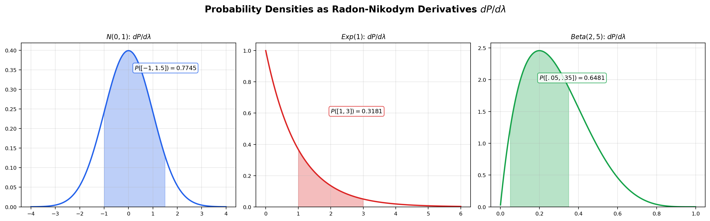
📝 Example 4 (The R-N derivative you already know)
Every probability density function the reader has ever computed with is a Radon-Nikodym derivative w.r.t. Lebesgue measure on . For the standard normal,
For the exponential distribution with rate ,
For the Beta distribution on ,
where is the Beta function. In each case the function on the right is the R-N derivative of the probability measure on the left with respect to Lebesgue measure on . The defining property becomes the familiar identity .
📝 Example 5 (Discrete R-N derivative is the PMF)
Let be counting measure on (assigning measure to each integer) and let be the geometric distribution with parameter , so . Then (any -null set is empty), and the R-N derivative is
The defining property reduces to for . The R-N derivative of a discrete probability measure with respect to counting measure is exactly the probability mass function. The “PDF vs PMF” distinction every student learns is purely about which dominating measure you take the derivative against — Lebesgue for continuous distributions, counting for discrete ones. The Radon-Nikodym framework unifies them.
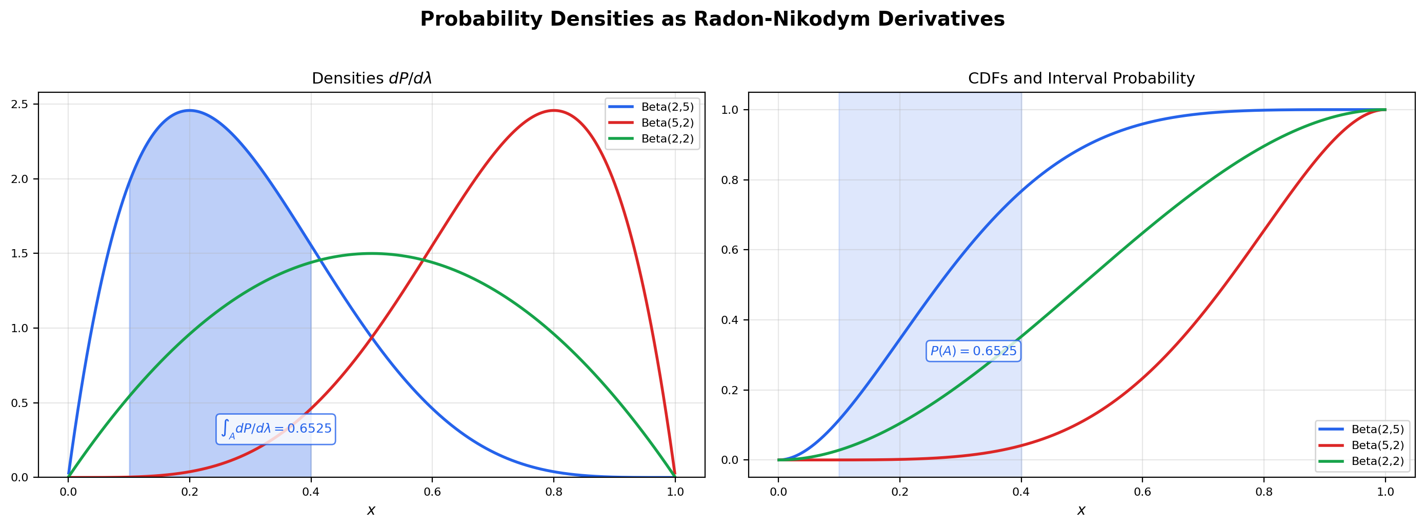
Drag the endpoint handles on the density panel to change the interval A = [a, b]. The R-N derivative dP/dλ is the density curve on the left; integrating it over A recovers the probability P(A), which equals the difference of CDF values F(b) − F(a) on the right. The two computations agree to numerical precision — that's exactly what the Radon-Nikodym theorem guarantees.
4. The Radon-Nikodym Theorem
We have defined the R-N derivative and shown it is unique when it exists. The substance of the theory is the existence statement: whenever and both measures are -finite, the derivative exists. The proof uses the projection theorem from Topic 27 §9 — the very tool that section advertised as a forward reference. This is the proof Topic 27 promised.
🔷 Theorem 1 (Radon-Nikodym theorem)
Let be a -finite measure space and let be a -finite measure on with . Then there exists a non-negative measurable function such that
The function is unique -a.e. (Proposition 1) and is called the Radon-Nikodym derivative .
Proof.
Following von Neumann, we reduce the existence of the density to a single application of orthogonal projection. The argument has four stages.
Stage 1 — Reduction to finite measures. By -finiteness, we can write as a disjoint union with and for every . If we can produce a density on each — that is, a function with for every — then the function is a density for on all of . So it suffices to prove the theorem under the additional assumption that both and are finite. Assume from here on that and .
Stage 2 — The auxiliary measure . Define , the sum measure. Both and are absolutely continuous with respect to (every -null set is in particular a -null set and a -null set). Now consider the linear functional defined by
This is linear in . To check it is bounded, apply the Cauchy-Schwarz inequality in :
The last step uses pointwise as set functions. Now apply Cauchy-Schwarz to bound the integral by an integral:
So , which is exactly the statement that is a bounded linear functional on with operator norm at most .
Stage 3 — Riesz representation via projection. By Topic 27 §9 Proposition 3 — or equivalently the Riesz representation theorem for Hilbert spaces, which we previewed in Section 9 of that topic — every bounded linear functional on a Hilbert space is represented by an inner product with a unique element of the space. Applied to our on the Hilbert space , this gives a function such that
Combining with the definition of , we get the integral identity that drives the rest of the proof:
\int g \, d\nu = \int g h \, d\rho \quad \text{for every } g \in L^2(\rho). \tag{$\ast$}
This is the entire content of Topic 27’s projection theorem applied here. Everything in Stage 4 is bookkeeping that turns into the actual R-N derivative.
Stage 4 — Extract the derivative. Substitute in for an arbitrary measurable set (this is allowed because is finite, so ). The left side becomes , and the right side becomes . So
Rearranging,
\int_A (1 - h) \, d\nu = \int_A h \, d\mu \quad \text{for every } A \in \mathcal{F}. \tag{$\ast\ast$}
We claim -a.e. To see , choose in : the right side is (because on ), and the left side is (because on and is positive). Both being equal forces both to be zero, which forces and , hence . So -a.e. The argument that is symmetric: choose , observe that on while , and conclude both sides are zero so .
Now consider the set . Plugging into gives , hence (since on the set). By absolute continuity , this forces . So we may discard the set — it has both -measure zero and -measure zero — and assume on .
Define
Then everywhere (since ). The remaining step is to upgrade the test-function identity from indicators to functions large enough to invert — this is the only place the algebra needs care.
The integral identity — namely for every measurable — extends from indicators to non-negative measurable test functions by the standard machine: linearity gives it for simple functions, and the Monotone Convergence Theorem (Topic 26 Theorem 1) extends it to non-negative measurables. Equivalently, the two measures and on agree on every measurable set, hence are equal as measures.
Now apply this extended identity to the test function , where for some (so that is bounded by and hence integrable). On this restricted set the substitution gives
So for every . Taking and applying MCT to the increasing sequence extends the identity to all measurable . Combined with the earlier observation that , we get for every measurable .
This is exactly the Radon-Nikodym identity: is the density we sought. Finiteness of in follows from , since .
💡 Remark 3 (Why the von Neumann proof)
The classical proof of Radon-Nikodym (via the Hahn decomposition theorem) requires building two pages of signed-measure machinery from scratch — positive sets, negative sets, total variation, and the Hahn decomposition itself. Von Neumann’s proof reduces the entire theorem to a single application of projection, which we already proved in Topic 27. The argument is essentially: “a bounded linear functional on is representable as an inner product, and the R-N derivative falls out of the algebra.” This is one of the most elegant proof strategies in analysis. It also closes Topic 27’s promise: the projection theorem we previewed in §9 is the engine that drives this proof. The function-space machinery built one topic ago has paid off in full.
5. Properties of the Radon-Nikodym Derivative
The Leibniz notation is not a coincidence: R-N derivatives obey a chain rule and an inverse rule that mirror the behavior of classical derivatives. These properties make formal manipulations with R-N derivatives feel exactly like the change-of-variables computations from single-variable calculus — except that the “derivative” is now a function in instead of a number.
🔷 Theorem 2 (Chain rule for R-N derivatives)
Let , , and be -finite measures on with . Then and
Proof.
That follows immediately from the chain of implications: if then (by ), and then (by ). For the formula, let and , both of which exist by Theorem 1. We need to show for every , because then by uniqueness (Proposition 1), must equal a.e.
Start with the definition of : . We want to rewrite the right side as a -integral. The key fact is that for any non-negative measurable function ,
where . This identity follows by the standard machine: it holds for (just the definition of as the density), extends to simple functions by linearity, extends to non-negative measurables by the Monotone Convergence Theorem (Topic 26 Theorem 1), and extends to functions by the decomposition. Apply this with :
This holds for every measurable , so by Proposition 1, -a.e.
🔷 Proposition 2 (Inverse rule)
Let and be -finite measures on with and (mutual absolute continuity). Then
This follows from the chain rule with : , so the two factors are reciprocals where they are nonzero. Mutual absolute continuity guarantees that the set where one factor vanishes is a null set under both measures, so the reciprocal is well-defined a.e.
📝 Example 6 (Chain rule and the change-of-variables formula for densities)
Let be a real-valued random variable with density with respect to Lebesgue measure . Let be a strictly monotone differentiable function with nowhere-zero derivative — that is, a diffeomorphism of onto its image — and let . The pushforward measure has a density with respect to Lebesgue measure on the image. By the chain rule for R-N derivatives applied to the pushforward,
This is the change-of-variables formula for probability densities that every introductory probability course states without proof. The factor is the Jacobian of the inverse transformation, and the entire formula is just the chain rule for R-N derivatives applied in the special case of a bijection between two open subsets of . The same formula in higher dimensions involves the Jacobian determinant of the inverse map — again as an application of the chain rule, now for measures on .
💡 Remark 4 (The Leibniz notation is not a coincidence)
R-N derivatives satisfy a chain rule (Theorem 2), an inverse rule (Proposition 2), and — with the right definitions — a kind of product rule. This is exactly the algebra of classical derivatives, and the Leibniz-style notation was chosen to make the analogy explicit. But the analogy has a limit: the R-N derivative is an equivalence class of functions in (modulo -null sets), not a number. Identities like the chain rule hold -almost everywhere, not pointwise. When using R-N notation, always remember the “a.e.” qualifier — it is the price of generality, and dropping it is the most common bookkeeping error in measure-theoretic probability.
6. Signed Measures and Jordan Decomposition
So far we have only discussed positive measures (functions ). The Radon-Nikodym theorem extends to signed measures, which take values in (or , with at most one infinity allowed). We give the bare minimum needed to state the extension; the full Hahn decomposition theory is treated in Folland §3.1 for the reader who wants more.
📐 Definition 4 (Signed measure)
A signed measure on is a function that takes at most one of the values , satisfies , and is countably additive: for every disjoint sequence ,
Positive measures are the special case of signed measures that happen to take only non-negative values.
📐 Definition 5 (Total variation)
The total variation of a signed measure on is the positive measure defined by
where the supremum runs over all finite measurable partitions of . The total variation measures the total mass moved by , treating positive and negative contributions equally.
🔷 Theorem 3 (Jordan decomposition)
Every signed measure with can be written uniquely as
where and are positive (finite) measures with . Moreover, .
Proof.
We sketch the proof; the full Hahn decomposition argument is in Folland §3.1. The Hahn decomposition theorem (which we state without proof here) gives disjoint sets with such that for every measurable and for every measurable . Define
Both are positive measures by construction: is non-negative because , and is non-negative because on subsets of (so ). They are mutually singular because they live on disjoint sets ( and ). The sum recovers because . Uniqueness of the decomposition follows from the mutual singularity of and : any other pair of positive mutually-singular measures with the same difference must coincide with these on the sets and .
💡 Remark 5 (Why the minimal scope)
We keep signed-measure theory deliberately minimal because the primary applications in this topic — probability densities, conditional expectation, importance sampling — are about positive measures. Jordan decomposition appears here for two reasons. First, it gives the cleanest extension of the R-N theorem to signed measures: if is a signed measure with , then and , so applying Theorem 1 to each piece gives and , and we define as a function in . Second, the conditional-expectation construction in Section 9 applies to any random variable , not just non-negative ones — and that argument relies on the signed-measure version of R-N to handle properly.
7. The Lebesgue Decomposition Theorem
The Radon-Nikodym theorem assumes . What happens when we drop that assumption? The Lebesgue decomposition theorem says: any -finite measure splits canonically into an absolutely continuous part and a singular part. Together with R-N, this gives a complete picture: the absolutely continuous part has a density, and the singular part lives on a null set of .
🔷 Theorem 4 (Lebesgue decomposition theorem)
Let and be -finite measures on . Then decomposes uniquely as
where and . In particular, has a Radon-Nikodym derivative , and is concentrated on a -null set.
📝 Example 7 (The Cantor three-part decomposition)
The cleanest worked example is a measure built from three pieces of mismatched type. Let
on , where is Lebesgue measure restricted to , is the Dirac mass at , and is the Cantor measure (the probability measure whose CDF is the Devil’s staircase from Topic 25). Decompose with respect to Lebesgue measure on . The absolutely continuous part is
The singular part is
The Dirac component sits on the single point (Lebesgue measure zero), and the Cantor measure is supported on the Cantor set (also Lebesgue measure zero), so via the partition versus . The singular part itself can be split further into a discrete component (, atoms) and a singular continuous component (, no atoms but no density). The full Lebesgue decomposition of any -finite measure on has at most these three pieces: absolutely continuous, discrete, and singular continuous.
💡 Remark 6 (Lebesgue decomposition from the von Neumann proof)
The Lebesgue decomposition theorem can be read off the same von Neumann argument that proved Radon-Nikodym. Recall the function from Stage 3 of the proof, where . The set is exactly where the absolute-continuity argument forced ; on this set, lives on a -null set, which is the singular part. On , the algebra produced the density , which is the absolutely continuous part. So defining and gives the decomposition. The full derivation is in Stein and Shakarchi, Chapter 6.
![Three-panel: the absolutely continuous component (uniform density on [0,1]), the discrete atom (Dirac mass at 0), and the singular continuous Cantor staircase, plus the combined CDF showing all three contributions](/images/topics/radon-nikodym/cantor-decomposition.png)
8. Probability Densities as Radon-Nikodym Derivatives
We promised in Section 1 to explain what a probability density “really is.” Here is the answer, made precise. The point of this section is not new mathematics — Definition 6 is just Definition 3 specialized to probability measures — but the change of vocabulary. Once you read “probability density function” as “Radon-Nikodym derivative with respect to Lebesgue measure,” everything in elementary probability snaps into rigorous focus.
📐 Definition 6 (Probability density function (rigorous))
Let be a probability measure on with , where is Lebesgue measure on . The probability density function of is
the Radon-Nikodym derivative of with respect to Lebesgue measure. It satisfies (i) -a.e., (ii) , and (iii) for every Borel .
📝 Example 8 (Beta density as an R-N derivative)
The Beta probability measure on has
where is the Beta function. The integral is exactly the definition of . The shape of the density encodes how distributes mass relative to the uniform distribution: when , the density is constant and is uniform; when the mass shifts right; when or the density blows up at an endpoint. The viz in Section 3 lets the reader explore this dependence interactively.
📝 Example 9 (When no density exists)
The Cantor measure on is not absolutely continuous with respect to Lebesgue measure: is supported on the Cantor set , which has Lebesgue measure zero. So , and does not exist. Not every probability measure has a density — only the absolutely continuous ones. The Cantor measure is the canonical example of a probability measure on with no density: it is continuous (no atoms — every singleton has measure zero) but not absolutely continuous (it lives on a Lebesgue-null set). It is the singular continuous part of the Lebesgue decomposition. Discrete distributions (like the Poisson or geometric) also have no density with respect to Lebesgue, but they do have densities with respect to counting measure — see Example 5.
💡 Remark 7 (Density is always with respect to a reference measure)
The phrase “the density of the Poisson distribution is ” is shorthand for , where is counting measure on . The same Poisson measure has no density with respect to Lebesgue measure on — it is supported on the integers, which form a Lebesgue-null set. Always ask: “density with respect to what?” The answer is almost always “Lebesgue measure” for continuous distributions and “counting measure” for discrete ones, but the framework allows densities with respect to any dominating measure, and exotic choices (like the Cantor measure on ) are sometimes useful in advanced applications.
9. Conditional Expectation via Radon-Nikodym
This is the flagship application. Conditional expectation is the single most important object in measure-theoretic probability — the workhorse of regression, Bayesian inference, reinforcement learning, and stochastic calculus — and the Radon-Nikodym theorem is what makes it well-defined when conditioning on a continuous variable. We state the definition, prove existence, prove the four basic properties, and then prove the -best-predictor theorem that connects everything to regression.
📐 Definition 7 (Conditional expectation $E[X \mid \mathcal{G}]$)
Let be a probability space, an integrable random variable, and a sub--algebra. The conditional expectation of given is the (a.e.-unique) -measurable function satisfying
In words: has the same integral as over every set you can describe using only the information in .
🔷 Theorem 5 (Existence and uniqueness of conditional expectation)
Under the conditions of Definition 7, exists and is unique -almost everywhere.
Proof.
Define the signed measure on the sub--algebra by
Countable additivity of follows from the Dominated Convergence Theorem (Topic 26 Theorem 3). Then : if and , then because the Lebesgue integral over a null set is zero. Both measures are -finite on (since is finite). By the Radon-Nikodym theorem extended to signed measures via Jordan decomposition (Section 6), there exists a -measurable function with
This is -measurable by the way the R-N theorem produces densities (the derivative is constructed inside the function space tied to the -algebra), and it satisfies the defining property of conditional expectation. Set . Uniqueness -a.e. follows from Proposition 1 applied to .
🔷 Proposition 3 (Properties of conditional expectation)
Let and let be sub--algebras of .
(i) Linearity. a.e., for any constants .
(ii) Tower property. a.e. Conditioning twice on a coarser-and-finer pair collapses to conditioning once on the coarser one.
(iii) Conditional Jensen. If is convex and , then a.e.
(iv) Independence. If is independent of — meaning the -algebra generated by is independent of — then a.e. (the constant function equal to the unconditional mean).
All four properties follow directly from the defining integral identity by routine measure-theoretic arguments — see Billingsley §34.
🔷 Theorem 6 ($L^2$-best-predictor theorem)
Let and let be a sub--algebra. Then is the unique element of that minimizes
over all -measurable . Equivalently, is the orthogonal projection of onto the closed subspace .
Proof.
Let and . We claim is a closed subspace of . It is clearly a linear subspace. For closedness, suppose converges to in — that is, . By the Riesz-Fischer theorem from Topic 27, convergence implies a subsequence converges -a.e. Pass to that subsequence. Since each is -measurable and the pointwise a.e. limit of -measurable functions is -measurable (after redefining on a null set), is -measurable, hence .
Now apply the projection theorem from Topic 27 §9 Proposition 3: there exists a unique element minimizing , characterized by the orthogonality condition
Specializing for (note since is -measurable), the orthogonality condition becomes
This is exactly the defining property of conditional expectation. By the uniqueness in Definition 7, a.e. So is the projection of onto , which is the best predictor of given in the mean-squared sense.
📝 Example 10 (Conditional expectation of a bivariate normal)
Let be jointly normal with and covariance matrix
A direct computation (complete the square in the joint density) gives
This is a linear function of — the conditional expectation is the linear regression of on . With the notebook’s preset values , , , , the slope is , so
At , this gives (analytical), and the notebook’s slice-averaging numerical method recovers approximately (modulo discretization error). The flagship visualization below lets you see the same curve from three angles — slice averaging, projection, and the explicit R-N derivative — and verify that they all produce the same function.
💡 Remark 8 (Regression is conditional expectation)
The -best-predictor theorem says: among all functions of , the one that best predicts in mean-squared error is . Linear regression, polynomial regression, kernel regression, random forests, and neural networks are all attempting to approximate this single object. The R-N theorem is what guarantees that the object exists at all (the function might be exotic, but it is well-defined and integrable). The projection theorem from Topic 27 is what guarantees it is unique and optimal in mean-squared error. The training loss of a regression model is the squared distance from this projection, and successful training reduces the gap. Forward link: Regression.
Toggle the three views to see one curve from three angles. Slice averaging: cut the joint density into vertical slices, average Y in each slice, and connect the means. L² projection: this is the closest function of X (in mean-squared error) to Y. R-N derivative: E[Y | X = x] is the Radon-Nikodym derivative of ν(A) = ∫_A Y dP with respect to P, restricted to the σ-algebra generated by X. The amber curve is the same in every view — that's the whole point.
![Three-panel: a joint density heatmap with the conditional expectation E[Y|X] curve overlaid, the slice-averaging interpretation showing means at representative x-values, and an L² error comparison showing that E[Y|X] beats the constant predictor E[Y]](/images/topics/radon-nikodym/conditional-expectation.png)
10. Change of Measure and Importance Sampling
The change-of-measure identity is the operational use of R-N derivatives that ML practitioners encounter most often: it is the engine of importance sampling, REINFORCE policy gradients, and the variational lower bound. The identity is short, the proof is the standard “indicator → simple → non-negative measurable → general” machine, and the consequences are everywhere. When the importance weights become unbounded, the Hoeffding tail bound used to certify importance-sampling accuracy collapses and one falls back to Chebyshev with the variance of the weights — exactly the Markov → Chebyshev → Hoeffding gap analyzed in Probability & The Union Bound.
🔷 Theorem 7 (Change of measure)
Let be -finite measures on with , and let be a -integrable function. Then
Integration with respect to is the same as integration with respect to after multiplying the integrand by the R-N derivative.
Proof.
Start with for . The left side is . The right side is
where the last step is the defining identity of the R-N derivative. So the identity holds for indicators. By linearity, it extends to simple functions . By the Monotone Convergence Theorem (Topic 26), it extends to non-negative measurable functions: any such is the increasing limit of simple functions , and both sides of the identity pass to the limit. Finally, for general -integrable , write with and apply the identity to each piece separately. The change-of-measure identity is the indicator-simple-monotone-linear chain in its purest form.
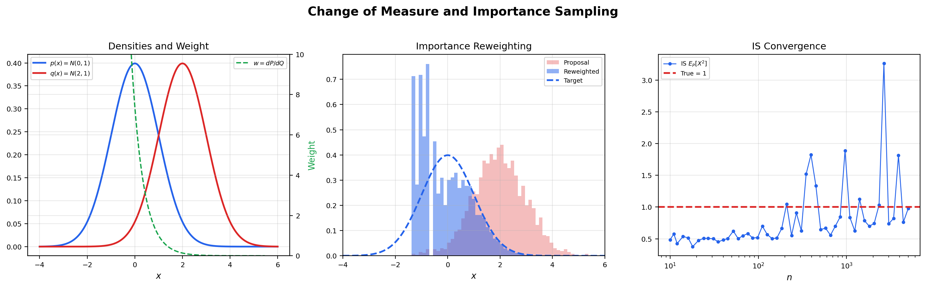
📝 Example 11 (Importance sampling)
Goal: estimate where is a target distribution that is hard or expensive to sample from, using samples from a proposal distribution that is easier. The change-of-measure identity gives
where is the importance weight. The estimator on the right is unbiased for as long as everywhere is integrable.
The notebook’s preset case takes , , and (so ). The weight has the closed form
The notebook generates samples from and computes the running estimate as grows; the trace converges to but the convergence is noisy because shifts the proposal away from the bulk of , blowing up the variance of the weights for negative . The interactive visualization below lets you watch this convergence directly and compare different target/proposal pairs.
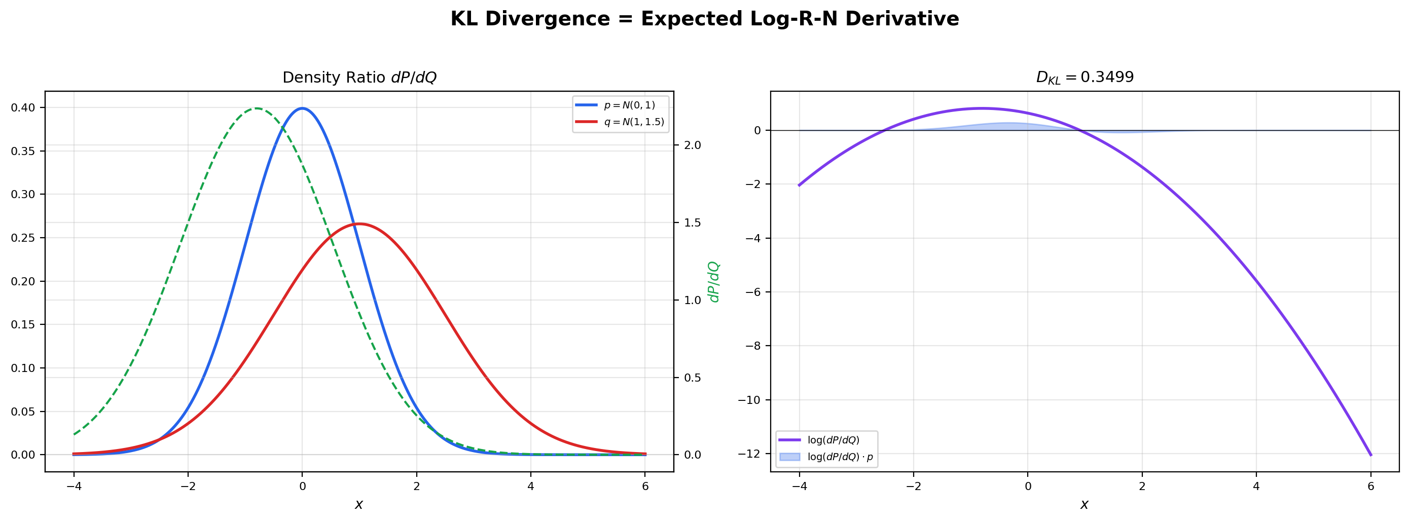
📝 Example 12 (KL divergence as expected log-R-N derivative)
The Kullback-Leibler divergence between two probability measures with is
It is the expected log-density-ratio under . Non-negativity follows from Jensen’s inequality (Topic 27 Theorem 1) applied with (which is convex):
The middle inequality is Jensen, and the last step uses the change-of-measure identity:
For two normal distributions and , the closed form is
The notebook verifies this analytic value against direct numerical integration of the integral , getting a match to \sim$$10^{-6}.
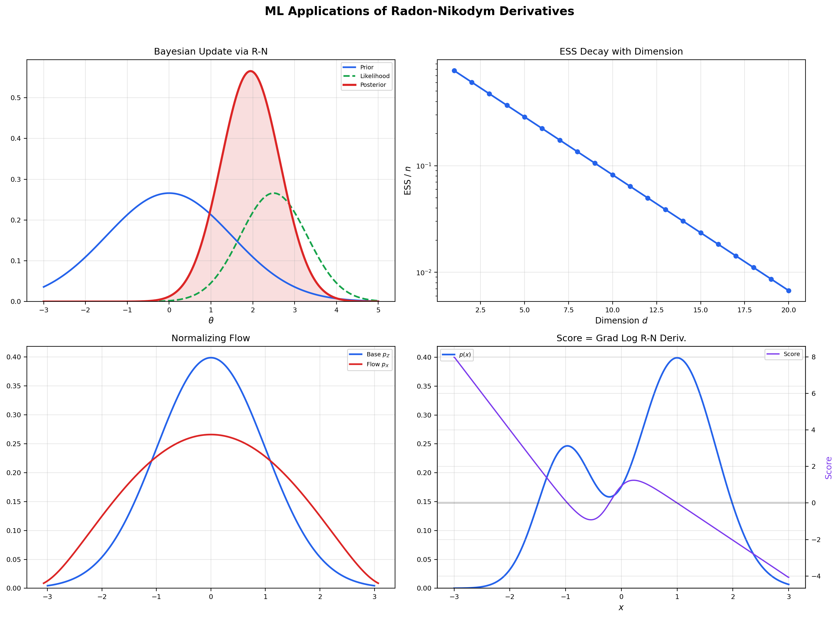
💡 Remark 9 (Normalizing flows are R-N chain rules in disguise)
A normalizing flow defines a bijection and pushes a base distribution (typically standard normal) forward to a learned distribution . The R-N derivative of with respect to Lebesgue measure on is computed via the chain rule for densities (Example 6 in higher dimensions):
This is the change-of-variables formula for densities, and it is just the chain rule for R-N derivatives applied to the pushforward measure. Normalizing flows are designed so that the determinant on the right is cheap to compute — coupling layers, autoregressive flows, and continuous flows are all architectural tricks for keeping tractable while preserving expressivity. Forward link: Generative Modeling.
Estimate E_P[f] using samples from the proposal Q. The importance weight w(x) = dP/dQ is a Radon-Nikodym derivative — the function that converts integration with respect to Q into integration with respect to P. The running estimate (slate) converges toward the true value (indigo dashed) as n grows. The effective sample size (ESS) measures how many of the n samples are doing meaningful work — an ESS far below n means the proposal is poorly matched to the target and most of the variance is concentrated in a few high-weight points.
11. Computational Notes
A few practical observations about computing R-N derivatives in code, since ML practitioners encounter them constantly under different names.
-
Kernel density estimation as R-N approximation. Given samples from a probability measure with , the kernel density estimator is a non-parametric estimate of . Under regularity conditions on the kernel and the bandwidth , converges to the true density in as , , and . KDE is the simplest and most direct way to estimate an R-N derivative from samples.
-
scipy.statsand densities. Every continuous distribution inscipy.statsexposes a.pdf(x)method that returns and a.logpdf(x)method that returns . The.logpdfform is preferred for numerical work because density values can be very small and underflow, but log densities are well-behaved across the entire support. -
Conditional expectation in pandas. A
df.groupby('X')['Y'].mean()call computes the empirical conditional expectation of given — that is, the slice average of over the groups defined by distinct values. This is the empirical version of the slice-averaging interpretation in Section 9, applied to a finite sample. -
Importance weights in PyTorch.
torch.distributions.Normal(0, 1).log_prob(x)returns for the standard normal density. The log-importance weight for samples from used to estimate expectations under islog_p(x) - log_q(x), which is . The actual weight isexp(log_p(x) - log_q(x)), but the log form is preferred until the very last step to avoid overflow.
📝 Example 13 (Numerical density-ratio verification)
For and , the density ratio has the closed form
Pick the integrand and verify the change-of-measure identity numerically by computing both sides of via quadrature on . Both integrals should agree to \sim$$10^{-6} — the expected accuracy of scipy.integrate.quad for smooth integrands. If they disagree by more than discretization error, either the weight is wrong or the support of extends beyond the support of (in which case and the identity does not hold). The notebook performs this verification step explicitly and confirms the agreement.
12. Connections to Machine Learning
This section is longer than the ML-connections sections in Topics 25–27, reflecting the extraordinary breadth of Radon-Nikodym applications in machine learning. Once you read “the density of ” as “the R-N derivative ,” every probabilistic computation in ML traces back to a change of measure or a conditional expectation.
Probability densities and likelihoods. Every PDF the practitioner has ever written down — Gaussian, Beta, Dirichlet, mixture model, neural-network output — is . Every likelihood is a product of R-N derivative values. Maximum likelihood estimation, Fisher information, and the Cramér-Rao bound all operate on R-N derivatives. The entire parametric statistics framework is built on this single object. Forward link: Probability Spaces.
Conditional expectation and regression. is the best predictor of given (Theorem 6), and it is an R-N derivative on a sub--algebra (Theorem 5). Least-squares regression, random forests, gradient-boosted trees, and neural-network regression are all approximating this single object. The normal equations of OLS are exactly the orthogonality condition from the projection theorem applied to the linear subspace of affine functions of . Forward link: Regression.
Bayesian inference as change of measure. Bayes’ theorem says the posterior density is proportional to the prior times the likelihood: . In R-N terms, the posterior measure is absolutely continuous with respect to the prior , and the R-N derivative is the (normalized) likelihood ratio. The posterior update is a change of measure from prior to posterior, and the normalization constant is the marginal likelihood. Variational inference, MCMC, and Hamiltonian Monte Carlo are all algorithms for working with this change of measure when the posterior cannot be computed in closed form. Forward link: Bayesian Inference.
Importance sampling and REINFORCE. The identity from Section 10 is the engine of importance sampling. In reinforcement learning, the REINFORCE policy-gradient estimator uses the same identity in disguise: , where the gradient is the score function — the gradient of the log R-N derivative. Every time a policy gradient is estimated by sampling from the current policy, an R-N derivative is being approximated. Forward link: Importance Sampling.
KL divergence and information geometry. is the expected log-R-N derivative. The Fisher information matrix is the covariance of the score vector — the gradient of the log R-N derivative — and it is the local curvature of the manifold of probability distributions in the KL geometry. Natural-gradient methods, mirror descent, and trust-region policy optimization all use this geometry. Forward link: Information Geometry.
Normalizing flows and diffusion models. Normalizing flows compute via the R-N chain rule applied to a learned bijection (Remark 9). Diffusion models learn the score at each noise level — the gradient of the log R-N derivative of the noisy data distribution — and use it to reverse the noising process. Both frameworks are built on R-N derivatives all the way down. Forward link: Diffusion Models.
-divergences and GANs. Every -divergence is a functional of the R-N derivative. KL is the special case . The total variation, Jensen-Shannon, , and Hellinger divergences are other choices of . Generative adversarial networks (GANs) train a discriminator that approximates , and the generator’s loss is some -divergence between the two distributions — the discriminator literally learns the R-N derivative. Forward link: Generative Modeling.
📝 Example 14 (Score function identity)
For a parametric family with densities , the score function is . A foundational identity says it has mean zero under :
Proof: differentiate with respect to . Under regularity conditions (those that justify swapping the derivative and the integral via the Dominated Convergence Theorem from Topic 26),
The middle step uses the chain rule for derivatives and the fact that where the support lies. This identity is the basis of maximum-likelihood asymptotics — the score is a martingale at the true parameter, and the variance of the score is the Fisher information.
📝 Example 15 (Variational lower bound (ELBO))
In variational inference, the marginal log-likelihood is intractable because it requires integrating over a latent variable : . The evidence lower bound (ELBO) sidesteps this by introducing an auxiliary distribution over the latents and applying Jensen’s inequality to the log:
The ratio inside the log is the R-N derivative of the joint with respect to the product of the data marginal and the variational distribution — a change of measure between two probability spaces. The ELBO is itself an expectation of a log R-N derivative, and maximizing it with respect to both the model parameters and tightens the bound on from below. Variational autoencoders, expectation maximization, and amortized inference all maximize ELBO objectives.
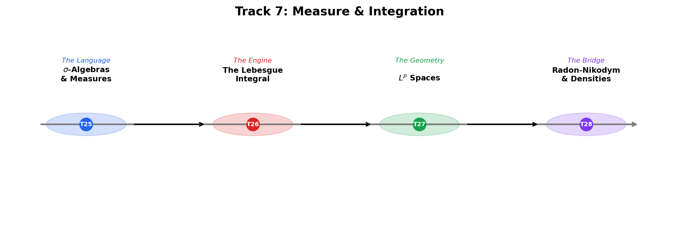
13. The Measure & Integration Arc — Closing Reflection
This is the fourth and final topic in the Measure & Integration track. The track tells a single story in four chapters. Topic 25 built the language: -algebras gave us a rigorous notion of “measurable set,” and measures assigned sizes to those sets in a way that is countably additive and well-behaved under countable operations. Topic 26 built the integral: the Lebesgue integral generalized Riemann’s by measuring the domain rather than the range, unlocking three convergence theorems (Monotone Convergence, Fatou, Dominated Convergence) that make limit/integral interchange rigorous. Topic 27 built function spaces: organized integrable functions into normed vector spaces with geometric structure — distances, balls, completeness — and the inner product made “projection onto a closed subspace” meaningful. Topic 28 completed the arc by turning measures into functions: the Radon-Nikodym theorem says that when one measure is absolutely continuous with respect to another, the relationship is captured by a single integrable function — the density.
The four topics form a chain of increasingly powerful tools. -algebras are the foundation (you cannot measure without them). The Lebesgue integral is the engine (you cannot integrate without it). spaces are the geometry (you cannot do analysis without norms and completeness). And the Radon-Nikodym theorem is the bridge to probability (you cannot do measure-theoretic probability without densities and conditional expectation). Each topic depends on the previous one, and the dependency is not formal — the proofs literally use the tools.
For the ML practitioner, this arc provides the rigorous underpinnings of the probabilistic tools used daily. The density is — a Radon-Nikodym derivative. The expected value is — a Lebesgue integral. The best predictor is an projection of the random variable onto the sub--algebra generated by . KL divergence is an integral of a log R-N derivative. Every probabilistic computation in modern machine learning traces back to this four-topic chain. The “Track 7” arc exists precisely so that a reader who finishes it can pick up any modern paper in measure-theoretic ML and recognize the pieces.
Connections & Further Reading
Prerequisites — topics you need first
Lp Spaces
The von Neumann proof of Radon-Nikodym uses L² orthogonal projection from Topic 27 Section 9. R-N derivatives live in L¹(μ). Topic 27's duality proof sketch used R-N as a black box — this topic closes that loop.
The Lebesgue Integral
The Lebesgue integral defines ν(A) = ∫_A f dμ, which is the relationship the R-N theorem reverses: given ν ≪ μ, recover f.
Sigma-Algebras & Measures
Measurable spaces, sigma-algebras, and null sets from Topic 25 are the framework. Conditional expectation uses sub-sigma-algebras.
Completeness & Compactness
Completeness of L² (Riesz-Fischer from Topic 27, which used the Bolzano-Weierstrass technique from Topic 3) ensures the closed-subspace projection exists.
Where this leads — next in formalCalculus
Normed & Banach Spaces
Lᵖ duality proved via Radon-Nikodym (now complete) is the canonical example of a dual-space characterization in functional analysis. The abstract dual-space theory, Hahn-Banach theorem, and the three pillars (UBP, Open Mapping, Closed Graph) build on this foundation.
Inner Product & Hilbert Spaces
Conditional expectation is the orthogonal projection of an L² random variable onto a sub-σ-algebra. The projection theorem provides existence and uniqueness, generalizing the von Neumann argument used here.
On to formalStatistics — where this calculus powers inference
Conditional Probability
The Radon–Nikodym theorem is exactly the existence proof for conditional expectation E[X|𝒢]: given a σ-finite measure P restricted to 𝒢 and the measure ν(A) = ∫_A X dP on 𝒢, the R-N derivative dν/dP|𝒢 is E[X|𝒢]. Conditional probability is its special case for indicator integrands.
Likelihood Ratio Tests And Np
The likelihood ratio Λ(x) = f_1(x)/f_0(x) = dP_1/dP_0 is the Radon–Nikodym derivative of the alternative w.r.t. the null. The Neyman–Pearson lemma — that the LRT is the most powerful test at any level — is proven using monotonicity properties of R-N derivatives.
Bayesian Foundations And Prior Selection
Posterior densities p(θ|x) are R-N derivatives of the posterior measure w.r.t. a dominating measure (Lebesgue on ℝ^d, counting on a countable set). Likelihoods L(θ;x) are R-N derivatives of the data measure across different θ. Bayes' rule is a change-of-measure identity.
Hypothesis Testing
The absolute-continuity assumption P_1 ≪ P_0 in hypothesis testing means the null assigns positive probability to every event of positive alternative probability — precisely the hypothesis of the Radon–Nikodym theorem. Without it, likelihood ratios are undefined on positive-probability events.
On to formalML — where this calculus powers ML
High Dimensional Regression
Conditional expectation $\mathbb{E}[Y \mid X]$ is the best $L^2$ predictor — the Radon–Nikodym derivative of a restricted measure — and least-squares regression computes it in $\mathbb{R}^n$. In the $p \gg n$ regime, the debiased lasso's $\sqrt n$-consistency proof uses the absolute-continuity hypothesis to make the conditional-density manipulations rigorous.
Information Geometry
KL divergence $D_\mathrm{KL}(P \| Q) = \int \log(dP/dQ)\,dP$ is the expected log-Radon–Nikodym derivative. Fisher information is the variance of the score, which is $\nabla \log(dP/d\lambda)$ for a fixed reference measure $\lambda$.
Density Ratio Estimation
§2.2's detour on absolute continuity uses the Radon–Nikodym theorem to ground the density-ratio function $r = dp/dq$ as a measurable object before the importance-weighting identity is applied; without it, the proof in Move 2 of §2.2 would be merely formal manipulation of $p/q$ on the set where the pointwise expression is undefined.
PAC Bayes Bounds
The Donsker–Varadhan variational form of KL divergence (§3.3 Theorem 1) depends on the existence of the Radon–Nikodym derivative $dQ/dP$ whenever $Q$ is absolutely continuous w.r.t. $P$. This is the technical condition that makes the master tool of §3 well-defined, and consequently every PAC-Bayes bound presumes $Q \ll P$ from §2.3 onward.
References
- book Royden, H. L. & Fitzpatrick, P. M. (2010). Real Analysis Fourth edition. Chapter 18 (Radon-Nikodym, Lebesgue decomposition). Closest to our von Neumann proof path.
- book Folland, G. B. (1999). Real Analysis: Modern Techniques and Their Applications Second edition. Chapter 3 (signed measures, R-N theorem, Lebesgue decomposition). Concise classical treatment.
- book Billingsley, P. (2012). Probability and Measure Anniversary edition. Chapters 31–33. Excellent for the probability interpretation — densities, conditional expectation, regular conditional distributions.
- book Stein, E. M. & Shakarchi, R. (2005). Real Analysis: Measure Theory, Integration, and Hilbert Spaces Chapter 6. Clean presentation of the von Neumann proof using L² projection.