Sigma-Algebras & Measures
Why not every set is measurable, and how the right framework for 'size' unlocks rigorous probability — from Borel sets to Lebesgue measure to the mathematical language that makes p(x) mean something precise.
Abstract. Measure theory is where analysis leaves the realm of pictures and becomes structural. The Riemann integral fails on important functions — the indicator of the rationals on [0,1] has no Riemann integral at all. To build a more powerful integral theory, we first need a more powerful notion of 'size.' A sigma-algebra tells us which sets we are allowed to measure; a measure assigns a non-negative number to each of those sets, respecting countable additivity. The Lebesgue measure on ℝ extends the intuitive notion of length to a far richer collection of sets than intervals — but the Vitali construction shows that not every subset of ℝ can be assigned a consistent measure. The measurable functions with respect to a sigma-algebra are precisely the functions for which integration will be defined. These concepts are the mathematical language of probability: a probability space is a measure space with total measure 1, and every density function, expectation, and convergence theorem in ML rests on this foundation.
1. Why the Riemann Integral Isn’t Enough
If this topic feels more abstract than the previous ones, that’s the subject matter, not your mathematical maturity — measure theory is where analysis becomes structural. Every prior topic in this curriculum has been geometric: epsilon-delta limits live near a point, derivatives are slopes, integrals are areas, vector fields are arrows, phase portraits are trajectories. Measure theory has none of those pictures. A sigma-algebra is a family of sets, and a measure is a function on that family. There is no picture of “the Borel sigma-algebra on ” — it is an uncountable collection of subsets that we can describe but never see.
That’s the bad news. The good news is that this abstract framework is what unlocks rigorous probability, modern analysis, and most of the mathematical machinery that machine learning silently depends on. By the end of this topic you’ll understand exactly what people mean when they write for a probability density, why “with probability 1” is more than a figure of speech, and why the Riemann integral you learned in calculus is not the right tool for any serious work in probability or functional analysis.
We’ll motivate the framework with three puzzles — each one a question the Riemann integral cannot answer.
Puzzle 1: The Dirichlet function
Define by
This is the indicator function of the rationals. Try to integrate it on via Riemann sums and you immediately hit a wall.
📝 Example 1 (The Dirichlet function has no Riemann integral)
Let be any partition of . On every subinterval — no matter how small — we can find both a rational point and an irrational point. So
Therefore the upper Darboux sum is and the lower sum is , regardless of the partition. The Riemann integral exists only when , but here the sup is and the inf is . The Riemann integral does not exist.
But our intuition is screaming that the integral should be . The rationals are countable; the irrationals are uncountable. Almost every point in is irrational, so is “almost everywhere zero.” A good theory of integration should recognize that. Measure theory will let us make “the rationals are negligible” a precise statement: has Lebesgue measure zero, so in the Lebesgue sense.
Puzzle 2: The Vitali impossibility
Suppose we want to assign a “length” to every subset . We’d want this length function to satisfy two reasonable properties:
- Translation-invariance: for any — sliding a set sideways doesn’t change its length.
- Countable additivity: for any countable collection of disjoint sets.
These look harmless. The shocking fact, due to Vitali in 1905, is that no such function exists — at least not one defined on every subset. We will prove this in Section 8: using the axiom of choice, we can construct a subset to which no consistent length can be assigned. The resolution is sobering: we don’t measure all subsets. We measure only those in a designated collection — a sigma-algebra. Choosing the right sigma-algebra is the central design choice of measure theory.
Puzzle 3: The ML density puzzle
When you write for the standard normal density, what does this mean operationally? The continuous random variable takes any specific value with probability zero — for every . So is not a probability. What is it?
The answer is that is a Radon-Nikodym derivative: it is the rate at which probability mass accumulates per unit Lebesgue measure. The expression "" means , where is the probability measure and is Lebesgue measure. Without measure theory, "" is a notational convenience with no operational content; with it, the relationship between and becomes precise. This connection is the entry point to the formalml.com topic on Probability Spaces.
These three puzzles all point to the same need: a framework where “size” is defined on a controlled family of sets, where countable operations behave well, and where the limitations of the Riemann integral can be transcended. That framework is built in the next eleven sections.
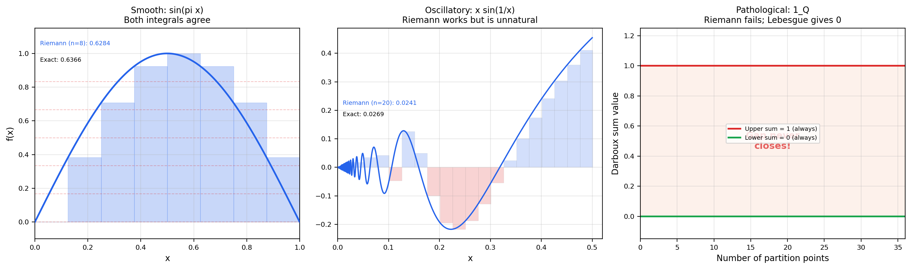
A smooth, well-behaved bump on [0, 1]. Both Riemann and Lebesgue integrals agree exactly with the closed form 2/π. Use this preset to see the two strategies converge in lockstep.
2. Sigma-Algebras
A sigma-algebra is a family of subsets of a fixed ambient set that is closed under complement, countable union, and contains itself. That’s it — three axioms. But these three axioms have surprisingly deep consequences, and choosing the right sigma-algebra is the central modeling decision of measure theory.
📐 Definition 1 (Sigma-algebra (σ-algebra))
Let be a non-empty set. A sigma-algebra on is a collection of subsets of satisfying:
- .
- Closure under complement. If , then .
- Closure under countable union. If is a countable sequence in , then .
The pair is called a measurable space. Members of are called measurable sets.
A few easy consequences fall out. Since and is closed under complement, . Closure under countable union plus complement gives closure under countable intersection (de Morgan). And since the union of a finite number of sets is a special case of a countable union (pad with ), is also closed under finite unions and finite intersections.
The simplest examples are at the two extremes: the smallest possible sigma-algebra and the largest possible one.
📝 Example 2 (The trivial sigma-algebra)
For any set , the collection is a sigma-algebra — the smallest one possible. Closure under complement is immediate ( and vice versa), and any countable union of these two sets is again one of these two sets. This sigma-algebra “knows” only whether a point is in or not — it carries no further information.
📝 Example 3 (The power set)
The full power set is a sigma-algebra — the largest one possible. It contains every subset of and is trivially closed under all set operations. When is countable, is the only sigma-algebra we ever use. But when , we will see that is too big — it contains pathological sets that no consistent length function can measure.
📝 Example 4 (A finite sigma-algebra from a partition)
Take and consider the partition and . The sigma-algebra generated by this partition is
This collection is closed under complement (the complement of is ) and under union (any union of the four sets is again in the four sets). Note that is not in — this sigma-algebra cannot distinguish from . It encodes precisely the information “which side of the partition does this point belong to?” and nothing more.
💡 Remark 1 (Sigma-algebras as 'levels of information')
The previous example hints at an interpretation that becomes essential in probability theory: a sigma-algebra is an abstract description of what information is available. A coarser sigma-algebra (fewer sets) corresponds to less information; a finer sigma-algebra (more sets) corresponds to more information. In the example above, knows only “is this point in or in ?” but not “is this point exactly ?” In probability, a filtration — a nested sequence of sigma-algebras — models information being revealed over time. This is the foundation of stochastic processes and the source of every “conditional expectation given ” in mathematical finance and reinforcement learning.
In practice, we rarely write down a sigma-algebra by listing its members. We specify a smaller collection of “interesting” sets and then close it up under the sigma-algebra axioms.
📐 Definition 2 (Generated sigma-algebra σ(C))
Let be any collection of subsets of . The sigma-algebra generated by , written , is the smallest sigma-algebra on that contains . Equivalently, it is the intersection of all sigma-algebras containing :
This intersection is non-empty (the power set always works) and is itself a sigma-algebra (the intersection of any family of sigma-algebras is a sigma-algebra — check the axioms). So is well-defined.
The most important generated sigma-algebra in all of analysis is the Borel sigma-algebra on the real line.
📐 Definition 3 (The Borel sigma-algebra B(ℝ))
The Borel sigma-algebra on , denoted , is the sigma-algebra generated by the collection of all open intervals:
Members of are called Borel sets. The collection contains every open set (each is a countable union of open intervals), every closed set (complements of open sets), every countable union of closed sets ( sets), every countable intersection of open sets ( sets), and so on through a transfinite hierarchy. In short: every “reasonable” subset of that you would write down without using the axiom of choice is Borel.
Equivalently, can be generated by any of the following: all open sets, all closed sets, all half-open intervals , all rays , all rationals as singletons. The choice of generator doesn’t matter — the resulting sigma-algebra is the same.
💡 Remark 2 (Why 'countable' and not 'finite' additivity)
The choice of countable (rather than finite) closure in the sigma-algebra axioms is the central technical decision of measure theory. With only finite closure, you get an algebra of sets — adequate for classical probability of dice and cards, but too weak for analysis. Countable closure is what makes limits behave correctly. For example, the set is the countable union of singletons for rational; in the Borel sigma-algebra it is automatically measurable, and its measure is the countable sum . With only finite additivity, this argument fails — the rationals would slip through the cracks. Countable additivity is exactly the right strength to make a.e. arguments, dominated convergence, and Fubini’s theorem all work.
3. Measures
A sigma-algebra tells us which sets we are allowed to measure. A measure tells us what number to assign to each one.
📐 Definition 4 (Measure on a measurable space)
Let be a measurable space. A measure on is a function satisfying:
- Non-negativity. for all .
- Empty set has measure zero. .
- Countable additivity. For any countable sequence of pairwise disjoint sets ,
The triple is called a measure space. When , the triple is a probability space and is a probability measure — usually denoted or .
Note that measures take values in the extended non-negative reals — sets of infinite measure are allowed, and their arithmetic obeys the conventions for and (the latter is a convention, not a theorem, but it makes integrals of functions on null sets behave correctly).
The three axioms force a number of properties to hold automatically — properties that mirror the geometric intuition of “area” or “length” in the real line. Together they form the toolkit you’ll use whenever you work with measures.
🔷 Theorem 1 (Basic properties of measures)
Let be a measure space. Then for all measurable sets :
- Monotonicity. If then .
- Subadditivity. (no disjointness required).
- Continuity from below. If is an increasing sequence with union , then as .
- Continuity from above. If is a decreasing sequence with intersection , and , then as .
Proof.
Monotonicity (1). Write as a disjoint union. Both and are measurable. By countable additivity (with all but two terms equal to ), since .
Continuity from below (3). Define a disjointified sequence: Each is measurable (difference of measurable sets), the are pairwise disjoint, and
By countable additivity applied to the disjoint , where the second equality is the definition of an infinite series and the third equality is finite additivity ( is the disjoint union of ).
Subadditivity (2). Disjointify as in (3): let and for . Then (so by monotonicity), the are pairwise disjoint, and . Countable additivity gives
Continuity from above (4). This reduces to (3) by taking complements relative to . The hypothesis is essential — see Royden §17.4 for the cautionary counter-example without finiteness.
Now for the canonical examples. These three measures are the workhorses of probability and analysis.
📝 Example 5 (Counting measure on ℕ)
Let and (every subset is measurable, since is countable). Define where if is infinite. This is the counting measure. It satisfies all three axioms: , , and the cardinality of a countable disjoint union is the sum of cardinalities. The counting measure is the foundation of discrete probability — every "" is integration against the counting measure.
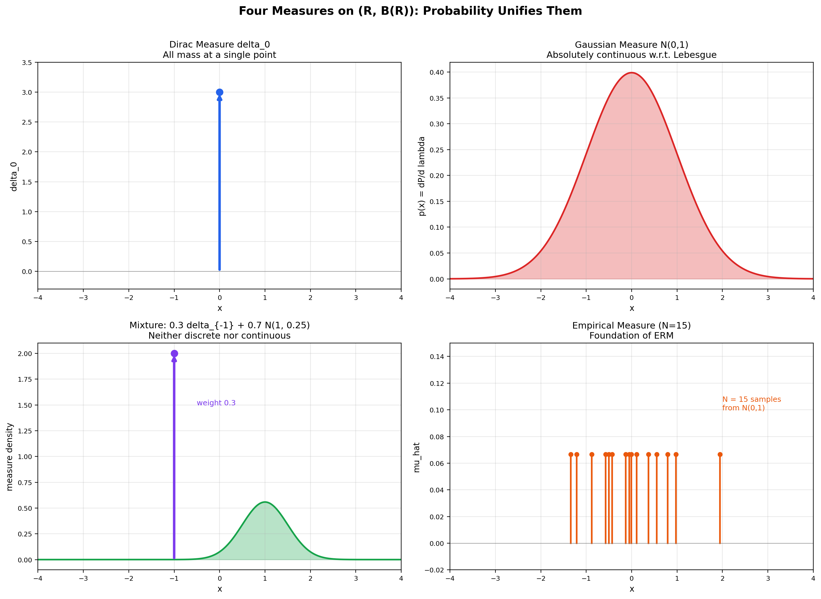
📝 Example 6 (Dirac measure δₐ)
Fix a point . The Dirac measure at is
This is a probability measure (, since ). Countable additivity holds because belongs to at most one set in any disjoint collection. Dirac measures are the building blocks of point masses in probability and the simplest non-trivial example of a singular measure with respect to Lebesgue measure on .
📝 Example 7 (Lebesgue measure on [0,1] (preview))
On the measurable space , there exists a unique measure such that for every interval . This is the Lebesgue measure on the unit interval, and constructing it rigorously is the work of Section 4 (we will need Carathéodory’s extension theorem). For now, observe that , so is a probability space — the uniform distribution on the unit interval.
💡 Remark 3 (Sigma-finite vs. finite measures)
A measure on is finite if and sigma-finite if can be written as a countable union with for every . Probability measures are finite. Lebesgue measure on is not finite () but is sigma-finite — write . Most theorems we care about (Fubini, Radon-Nikodym) assume sigma-finiteness; the non-sigma-finite case is where measure theory gets pathological. Throughout this topic, every measure is sigma-finite unless we explicitly say otherwise.
4. Lebesgue Measure on ℝ
We now construct the most important measure on the real line: the one that extends our intuitive notion of “length.” The construction is due to Lebesgue (1902) and Carathéodory (1914), and it proceeds in three stages: first define an outer measure on every subset of , then identify which subsets are measurable under that outer measure, and finally restrict to the measurable subsets to get a genuine countably additive measure.
📐 Definition 5 (Lebesgue outer measure λ*(A))
For any subset , the Lebesgue outer measure of is
The infimum is taken over all countable covers of by open intervals, and the value is the total length of the cover. Outer measure is defined for every subset of — but as we will see, alone is not countably additive on the full power set, so we need to restrict.
Some basic properties drop out immediately: (use the empty cover), is monotone (), is translation-invariant ( — translating a cover gives a cover of the translate with the same total length), and is countably subadditive (). What we don’t yet have is countable additivity on disjoint sets — and that requires choosing the right sigma-algebra to restrict to.
The crucial insight is Carathéodory’s: a set is “well-behaved” with respect to if it cleanly splits any other set into two pieces whose outer measures add up.
🔷 Theorem 2 (Carathéodory's extension theorem (statement))
A set is Carathéodory-measurable (with respect to ) if for every test set ,
Let denote the collection of all such measurable sets. Then:
- is a sigma-algebra containing every Borel set: .
- The restriction is a countably additive measure on .
- for every interval, recovering the geometric notion of length.
This restriction is the Lebesgue measure on , and is the Lebesgue sigma-algebra.
Proof.
The full proof is long — about ten pages in Royden — and we will not reproduce it here. The structural ingredients are:
- contains (trivially) and is closed under complement (the Carathéodory criterion is symmetric in and ).
- Closure under finite union follows from a careful inclusion-exclusion argument on the criterion.
- Closure under countable union uses both subadditivity of and continuity arguments to upgrade finite unions to countable.
- The fact that is countably additive on — the punchline — uses subadditivity in one direction and the Carathéodory criterion applied to disjoint sets in the other.
- The inclusion comes from showing every interval is Carathéodory-measurable, then using closure under countable operations to extend to all Borel sets.
For the complete argument, see Royden §2.4 or Folland §1.4. The takeaway for this topic is that is a strictly larger sigma-algebra than — every Borel set is Lebesgue-measurable, but there exist Lebesgue-measurable sets that are not Borel (their existence requires the axiom of choice). Both are smaller than , which contains the non-measurable Vitali set we will construct in Section 8.
📐 Definition 6 (Lebesgue measurable set)
A set is Lebesgue-measurable if it satisfies the Carathéodory criterion: for every , The collection of all such sets is the Lebesgue sigma-algebra , and is the Lebesgue measure on .
The next theorem captures the key invariance property — Lebesgue measure does not see translations. We give the full proof because it illustrates exactly how Carathéodory measurability propagates from to .
🔷 Theorem 3 (Translation-invariance of Lebesgue measure)
For every and every , the translate is also Lebesgue-measurable, and
Proof.
We split the proof into two parts: first that is translation-invariant on every subset of , then that is closed under translation.
Step 1: for every .
Let be any countable open cover of . Then is a countable open cover of with the same total length:
Taking the infimum over all covers of on the left and noting that every cover of produces a cover of of equal length (and vice versa, by translating by ), we get . So is translation-invariant on the full power set.
Step 2: If , then .
We must show that satisfies the Carathéodory criterion: for every ,
Apply Step 1 to translate by :
Now can be split using the measurability of (which we are given):
We translate each piece on the right side back by . Note that translated by gives , and translated by gives . By Step 1 again, translation does not change outer measure:
Substituting back:
This is exactly the Carathéodory criterion for , so . Step 1 then gives .
📝 Example 8 (λ([a,b]) = b - a — recovering interval length)
Let with . The interval is open-cover-able by for any , so . Taking gives . The reverse inequality is the non-trivial direction — it requires showing that no countable open cover of can have total length less than . The argument uses the Heine-Borel theorem (compactness of , from Topic 3) to extract a finite sub-cover, then a clean overlapping-intervals argument to bound the total length below by . Combined with the fact that is Borel and hence Lebesgue-measurable, we get .
📝 Example 9 (λ(ℚ ∩ [0,1]) = 0 — the rationals have measure zero)
The rationals in form a countable set: . For any , cover the -th rational by the open interval , which has length . The total length of this cover is
So for every , hence . Since is Borel (a countable union of singletons), it is Lebesgue-measurable, so .
This is the precise statement of “the rationals are negligible.” Combined with , we get that the irrationals in have measure — almost every point in the unit interval is irrational. The Dirichlet function is therefore zero almost everywhere with respect to Lebesgue measure, and its Lebesgue integral is — exactly what our intuition wanted in Section 1.
💡 Remark 4 (Lebesgue measure extends the Riemann integral)
A bounded function is Riemann-integrable if and only if its set of discontinuities has Lebesgue measure zero (Lebesgue’s criterion for Riemann integrability). For every Riemann-integrable , the Lebesgue integral exists and equals the Riemann integral. So Lebesgue integration is a strict extension of Riemann integration — it agrees with the old theory wherever the old theory applies, and assigns sensible values in many cases where the old theory fails (like the Dirichlet function).
![Outer measure covering: progressively refined interval covers of [0.3, 0.7]](/images/topics/sigma-algebras/outer-measure-covering.png)
Drag the endpoints (or the bar bodies) to reshape the intervals. The Lebesgue outer measure λ*(A) is the infimum of the total length over all countable open covers of A — so when the intervals cover A, their total length is at least λ(A) = 0.4. If you drag them so they no longer cover A, that lower bound no longer applies to the current arrangement. As you tighten a valid cover, the gap shrinks toward zero. Try "Optimize cover" to snap to a near-optimal arrangement.
5. The Cantor Set and Measure-Zero Surprises
The Cantor set is the single most important example in measure theory. It demonstrates that a set can be uncountable, closed, totally disconnected, and have Lebesgue measure zero — four properties that look incompatible until you see them coexist. The Cantor set is also the canonical example of a “fractal” — its construction predates Mandelbrot by seventy years.
📐 Definition 7 (The Cantor middle-thirds set C)
Define a sequence of sets recursively. Start with . To form , remove the open middle third of every interval in : and so on. The Cantor set is the intersection
After iterations, is a disjoint union of intervals each of length , so the total length of is . As , this length tends to zero — but the intersection is nevertheless non-empty and, as we will prove, uncountable.
🔷 Theorem 4 (The Cantor set is uncountable and has Lebesgue measure zero)
The Cantor set is a closed subset of that is:
- Uncountable — there is a bijection , so continuum.
- Of Lebesgue measure zero — .
Proof.
Measure zero. Since each has Lebesgue measure and for every , monotonicity of gives
Since as , the squeeze gives .
Uncountability. We use the ternary expansion characterization of . Every has a base-3 (ternary) expansion
The ternary expansion is unique except at terminating expansions, where the same number has two representations (analogous to in base 10). For terminating expansions we adopt the convention that ends in all ‘s when possible — this resolves the ambiguity.
The middle third removed at step is precisely the set of whose ternary expansion has (and cannot be replaced by ending in for any of these — the boundary points and themselves have alternative expansions with ). So consists of points with . By induction, consists of points whose first ternary digits are all in . Therefore
The map defined by sending to the binary sequence is a bijection. (It is well-defined and injective by the uniqueness of the chosen ternary expansion; it is surjective because every binary sequence corresponds to a valid ternary string in .)
By Cantor’s diagonal argument (Topic 3), is uncountable, with cardinality — the cardinality of the continuum. Therefore , and is uncountable.
📝 Example 10 (Fat Cantor sets with positive measure)
The standard middle-thirds Cantor set has measure zero because we remove a constant fraction at every step. If instead we remove a shrinking fraction at each step, we get a Cantor-like set with positive measure. Specifically, at step , remove a centered interval of length from each of the remaining intervals. The total length removed is
So the limiting set, the Smith-Volterra-Cantor set (or “fat Cantor set”), has Lebesgue measure . It is closed, nowhere dense, and uncountable — exactly like the standard Cantor set — but it has positive measure. This shows that “Cantor-like” does not imply “measure zero”: uncountability and measure zero are independent properties, and the standard middle-thirds set is a particular case where they happen to coincide.
💡 Remark 5 (The Cantor set is compact and totally disconnected)
is closed (it is the intersection of closed sets ) and bounded (a subset of ), so by Heine-Borel from Topic 3, is compact. It is also totally disconnected: between any two distinct points there is a deleted middle interval at some stage of the construction, so the connected components of are single points. A non-empty compact totally disconnected metric space without isolated points is called a Cantor space, and the Cantor set is the prototype. (Every two such spaces are homeomorphic — the Cantor set is, up to homeomorphism, the Cantor space.)
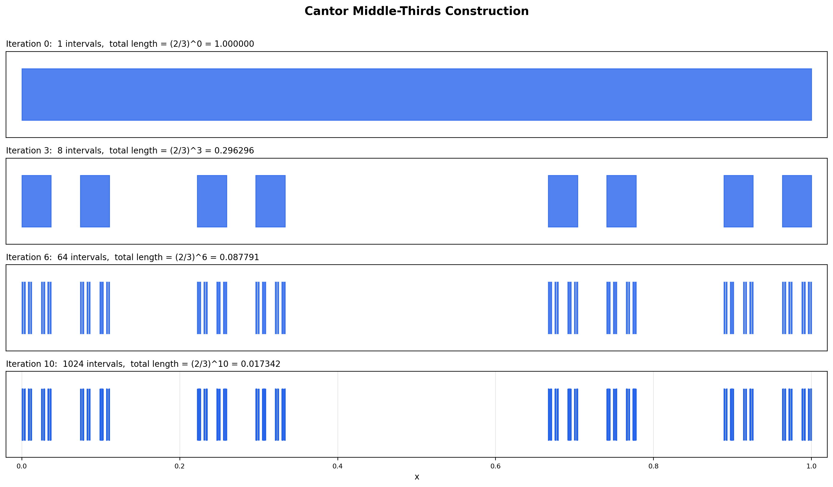
Standard middle-thirds set: at every step, remove the open middle 1/3 of each remaining interval. After 5 iterations, the total length is (2/3)^5 = 0.131687. The limiting set is non-empty and uncountable — every ternary expansion in {0, 2}^ℕ gives a point in C — yet it has total length 0.
6. Measurable Functions
Measurable functions are the class of functions for which the Lebesgue integral will be defined. The definition is suspiciously simple: a function is measurable if the preimage of every Borel set is measurable.
📐 Definition 8 (Measurable function)
Let be a measurable space. A function is -measurable (or just measurable when the sigma-algebra is clear from context) if for every Borel set ,
Equivalently — and this is usually how you check it in practice — is measurable if and only if for every . The “if” direction follows from the fact that the half-rays generate , and preimages commute with countable set operations.
The two universal examples are the continuous functions and the indicator functions.
📝 Example 11 (Continuous functions are Borel-measurable)
If is continuous and is open, then is open, hence Borel, hence Lebesgue-measurable. Since the open sets generate and preimages preserve countable set operations, for every Borel . So every continuous function is Borel-measurable. This is why the integral of a continuous function on a compact interval — the bread and butter of single-variable calculus — is just a special case of the Lebesgue integral.
📝 Example 12 (The Dirichlet function is Borel-measurable)
The indicator takes only two values, so its preimage of any Borel set is one of , , , or , depending on which of and lie in . All four sets are Borel ( is a countable union of singletons), so is Borel-measurable. Combined with our earlier observation that , this is the foundation for showing — once we have built the integral in Topic 26.
The Lebesgue integral of a measurable function is built up in two steps. First we define the integral for “simple functions” — finite linear combinations of indicators — and then we extend to general non-negative measurable functions by approximating from below.
📐 Definition 9 (Simple function)
A measurable function is simple if it takes only finitely many values. Equivalently, has a representation where are distinct real numbers and is a finite measurable partition of (each is measurable, the are pairwise disjoint, and ). The integral of a non-negative simple function with respect to a measure is defined to be
(With the convention , this is well-defined even when some but .)
The next theorem is the engine of Lebesgue integration: every non-negative measurable function is the pointwise limit of an increasing sequence of simple functions. Once you have this, the integral of a general non-negative measurable function can be defined as the limit of the integrals of the approximating simple functions.
🔷 Theorem 5 (Simple function approximation (dyadic construction))
Let be a non-negative measurable function. Then there exists a sequence of non-negative simple measurable functions such that:
- (the sequence is monotone increasing).
- for every .
- The convergence is uniform on every set where is bounded.
Proof.
We construct explicitly via dyadic slicing of the range. For each , partition the interval into dyadic subintervals of length :
Define
Each is a finite sum of step values times indicators of preimage sets, so it is a simple function. Each preimage set is measurable (preimage of a Borel set under a measurable function), so is measurable.
Monotonicity (). Suppose for some . Then . The next-finer dyadic partition splits this interval in half: lies in either or . In the first case . In the second case . Either way . The case where (the “cap”) is handled similarly: increasing either keeps at the cap or moves it into a finer dyadic level above .
Pointwise convergence (). Fix . If , choose so large that . For all , for some in the dyadic partition, so
Hence . If , then for every , so .
Uniform convergence on bounded sets. If on a set , then for we have for all , and the bound holds uniformly in . So uniformly on .
💡 Remark 6 (Simple function approximation partitions the range)
Theorem 5 is the constructive heart of Lebesgue integration. Notice what it does: it slices the range of into dyadic levels and uses the preimages of those levels as the building blocks for simple functions. This is the exact opposite of the Riemann strategy, which slices the domain into uniform subintervals. The Riemann approach fails on the Dirichlet function because no domain partition can separate rationals from irrationals; the Lebesgue approach succeeds because the range of has only two values and their preimages ( and its complement) are both Borel-measurable. The “partition the range” insight is the single most important conceptual move in measure theory, and it is what makes the Lebesgue integral strictly more powerful than the Riemann integral.
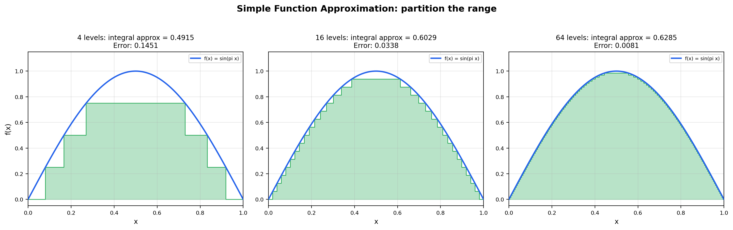
Dyadic simple function: slice the y-axis into 16 levels, and on each level, color the preimage A_k = {x : f(x) ∈ [k/16, (k+1)/16)·max}. The simple function s(x) = Σ c_k · 1_{A_k} is the largest dyadic step function below f. As you increase the level count, s converges to f from below — this is the constructive heart of Theorem 5 (simple function approximation).
7. Null Sets and “Almost Everywhere”
Once we have measures, we can make precise the language of “ignoring negligible sets” — the language of statements that hold “almost everywhere” or “with probability 1.” This is the vocabulary every probability theorem uses.
📐 Definition 10 (Null set (measure-zero set))
Let be a measure space. A set is a null set (or -null set) if . Examples on : every singleton , every countable set (such as ), and the Cantor set .
📐 Definition 11 (Almost everywhere (a.e.))
A property is said to hold almost everywhere with respect to — written -a.e. or simply a.e. when the measure is clear — if the set of for which fails is contained in a null set:
In probability, where is a probability measure, “almost everywhere” is usually called almost surely, abbreviated a.s. or “with probability .” When you read “the gradient flow converges to a critical point with probability 1,” the “with probability 1” is the measure-theoretic statement that the bad set has Lebesgue measure zero.
📝 Example 13 (The Dirichlet function is zero almost everywhere)
On the rationals form a null set (, by Example 9). So and the almost-everywhere equivalence class of is the same as that of the constant zero function. Once we have the Lebesgue integral, this will give — exactly the answer our intuition demanded back in Section 1.
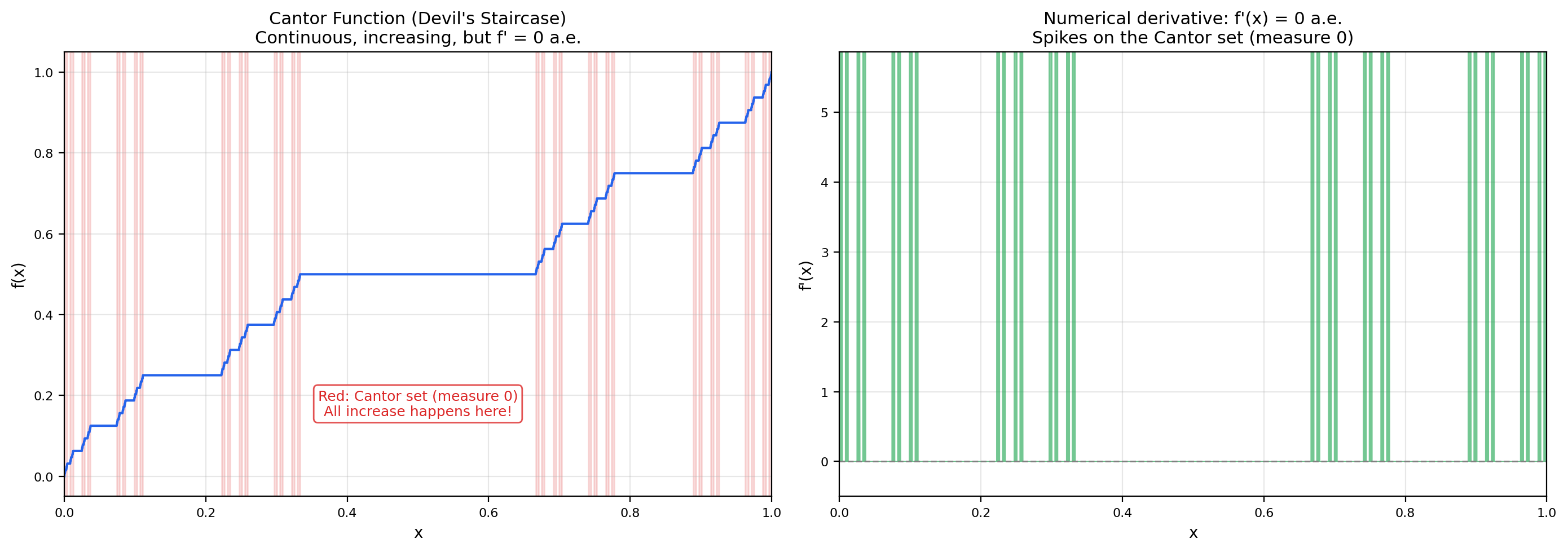
📝 Example 14 (The Cantor function (devil's staircase))
There exists a function , called the Cantor function or devil’s staircase, with the following remarkable properties:
- is continuous.
- is non-decreasing, with and .
- is differentiable almost everywhere with a.e.
The construction is iterative: is constant on every “removed middle third” of the Cantor set construction (taking the value on , the values and on the next two removed middles, and so on). On the Cantor set itself, is defined by a base--to-base- digit substitution.
The “missing increase” paradox is striking: goes from to continuously, yet its derivative is almost everywhere. All of the “increase” happens on the Cantor set , which has measure zero. The fundamental theorem of calculus fails for :
The FTC requires absolute continuity, and the Cantor function is the canonical example of a continuous, non-decreasing function that is not absolutely continuous. This is exactly the kind of pathology that motivates measure theory — the Riemann picture cannot detect the difference, but the measure-theoretic picture can.
💡 Remark 7 ('Almost everywhere' is relative to a measure)
The property “-almost everywhere” depends entirely on which measure you have in mind. The set has Lebesgue measure zero (so Lebesgue-a.e.), but it has counting measure (so counting-a.e.). When you read or write “a.e.” in measure theory, always know which measure you mean — switching measures changes which sets are negligible.
📐 Definition 12 (Complete measure)
A measure on is complete if every subset of every null set is itself measurable (and therefore also has measure zero). Equivalently, if with and , then . A measure is incomplete if there exists a null set with a non-measurable subset.
💡 Remark 8 (Borel vs. Lebesgue — completeness via completion)
The Borel sigma-algebra is not complete: there exist subsets of the Cantor set that are not Borel, for a cardinality reason. The Cantor set has cardinality , so its power set has cardinality — strictly larger than . There are more subsets of than there are Borel sets in total, so most subsets of are not Borel. The Lebesgue sigma-algebra is the completion of with respect to Lebesgue measure: it contains every Borel set plus every subset of every Lebesgue-null set. Lebesgue measure , restricted to , is complete by construction. In practice, completeness rarely matters for theorems we care about (the dominated convergence theorem doesn’t require it), but it eliminates pathological “this set is null but its subsets aren’t measurable” annoyances.
8. Non-Measurable Sets — The Vitali Construction
We have spent six sections building Lebesgue measure on a carefully chosen sigma-algebra. We can now answer the question that started this topic: why do we need to restrict to a sigma-algebra at all? Why not just measure every subset of ?
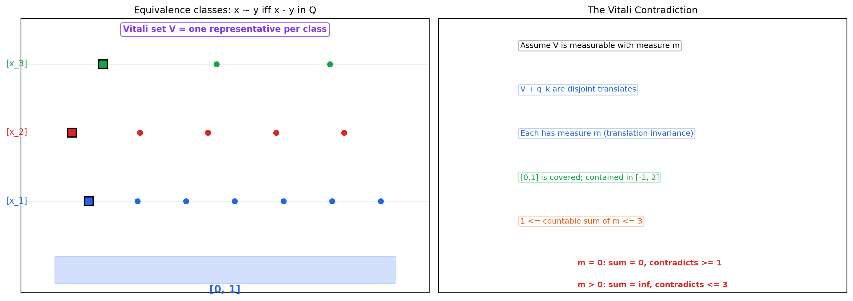
The answer is the Vitali construction. Using the axiom of choice, we can build a subset to which no consistent length can be assigned — assuming “consistent” means translation-invariant and countably additive. This is one of the most important (and most disquieting) results in classical analysis.
🔷 Theorem 6 (Existence of a non-Lebesgue-measurable set (Vitali, 1905))
There exists a subset such that . That is, is not Lebesgue-measurable.
Proof.
Define an equivalence relation on by
This is reflexive (), symmetric ( iff ), and transitive (). So partitions into equivalence classes — each class is the intersection for some real number , which is countably infinite (uncountably many distinct classes).
By the axiom of choice, we can select exactly one representative from each equivalence class. Let be the resulting set of representatives.
We claim is not Lebesgue-measurable. Suppose for contradiction that it is, with measure .
Enumerate the rationals in as (a countable set). Consider the translates for . We make two observations.
Disjointness. Suppose for some . Then for some , so , meaning . But contains exactly one representative of each equivalence class, so , which gives , contradicting . Hence the translates are pairwise disjoint.
Coverage. For any , the equivalence class has a representative . Then , where . So for some , and . Hence
By countable additivity (the translates are disjoint and measurable, since is assumed measurable and Lebesgue measure is translation-invariant by Theorem 3),
By monotonicity,
Now examine the cases:
- If , the sum , contradicting .
- If , the sum , contradicting .
Either way we have a contradiction. So our assumption that is measurable was false: .
💡 Remark 9 (The axiom of choice is essential — Solovay (1970))
The Vitali construction critically depends on the axiom of choice — without it, we cannot “select one representative from each equivalence class.” This raises a natural question: is the existence of non-measurable sets a theorem of ZFC, or is it an artifact of the axiom of choice? The answer, due to Solovay (1970), is striking: there exists a model of Zermelo-Fraenkel set theory (without choice, but with a weaker axiom of “dependent choice”) in which every subset of is Lebesgue-measurable. So non-measurable sets are not a feature of the real line itself — they are a consequence of the strong choice principle that mathematicians have collectively decided to adopt. In a universe without the full axiom of choice, the entire Vitali pathology vanishes, and Lebesgue measure extends to every subset.
The pragmatic upshot: in everything we do in measure theory and probability, we work with the axiom of choice, accept that non-measurable sets exist, and quietly restrict all our attention to the Borel or Lebesgue sigma-algebra. The non-measurable sets are out there, but the theorems we care about never need them.
9. Product Measures (Preview)
To integrate functions of two or more variables, we need to combine measures on different spaces into a product measure on the Cartesian product. The full theory — including Fubini’s theorem, which lets us compute double integrals as iterated integrals — belongs to The Lebesgue Integral. Here we lay the foundation.
📐 Definition 13 (Product sigma-algebra)
Let and be measurable spaces. The product sigma-algebra on , denoted , is the sigma-algebra generated by all “rectangles” with and :
📝 Example 15 (The Borel sigma-algebra on ℝ² is the product of two copies of B(ℝ))
On the plane , the Borel sigma-algebra generated by all open sets equals the product sigma-algebra . This is because every open set in can be written as a countable union of open rectangles , and conversely every open rectangle is open in . So the two ways of building “Borel sets in the plane” — directly from the topology, or as a product of one-dimensional Borel sigma-algebras — give the same answer. The same holds in arbitrary dimension: .
💡 Remark 10 (Joint distributions as product measures)
In probability theory, if and are independent random variables on a probability space , then their joint distribution is the product measure on . The product structure is the formal definition of independence: for any Borel sets ,
This is the measure-theoretic foundation of every “i.i.d.” assumption in machine learning. When you train a model on data points assumed i.i.d. from a distribution, you are implicitly working with a product measure over the data space.
10. Computational Notes
Measure theory is a foundational subject — most of what we have covered is non-computational. But the framework has direct algorithmic counterparts in scientific Python that practitioners use every day, often without realizing they are doing measure theory.
Monte Carlo estimation of Lebesgue measure. For a Borel set , the Lebesgue measure can be estimated by sampling independent uniform points and computing
By the strong law of large numbers, almost surely as . The central limit theorem gives the convergence rate: the standard error is . This is exactly the same rate as Monte Carlo integration of any bounded function — measure estimation is integration of an indicator function.
scipy.stats is measure theory in disguise. Every distribution object in scipy.stats is, mathematically, a probability measure on . The .pdf() method returns the Radon-Nikodym derivative of the distribution with respect to Lebesgue measure (when the distribution is absolutely continuous). The .cdf() method returns the measure of the half-line :
from scipy.stats import norm
norm.cdf(1.96) - norm.cdf(-1.96)  # ≈ 0.95
This is the measure-theoretic statement where is the standard normal measure.
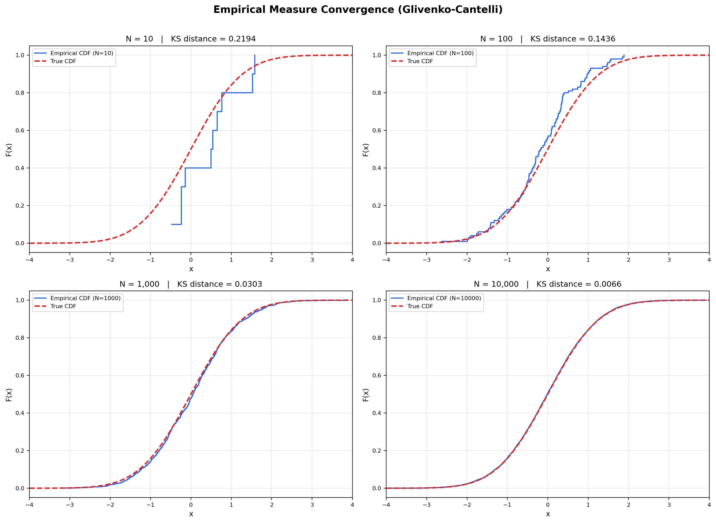
Empirical measures in PyTorch. The empirical measure of a finite sample is where each is the Dirac measure at . This is a probability measure on that puts mass at each sample point and zero elsewhere. Empirical risk minimization — the workhorse of supervised learning — is precisely the minimization of over a hypothesis class . The fact that this approximates the true population risk is the Glivenko-Cantelli theorem, a measure-theoretic statement we will see in Section 11.
Numerical pitfall: floating-point measure-zero detection. Measure-zero properties are asymptotic and inherently invisible to finite-precision arithmetic. A floating-point random sample from any continuous distribution will, with probability one, never land on any specific countable set — but a finite sample of size contains exactly points, all rational (every IEEE-754 double is rational). The “set of irrationals” is mathematically well-defined and has measure on , but no Python program can ever directly check whether a sampled is in it. Measure-zero subtleties live in the limits, not in the sampled data.
📝 Example 16 (Monte Carlo estimation of λ([0.3, 0.7]))
We want to estimate the measure of , which we know is .
import numpy as np
N = 10**6
samples = np.random.uniform(0, 1, N)
estimate = np.mean((samples >= 0.3) & (samples <= 0.7))
print(estimate)  # ≈ 0.4000
Running this with gives an estimate within of the true value, consistent with the predicted standard error . As grows, the empirical proportion converges to the true Lebesgue measure — this is Glivenko-Cantelli in its most elementary form.
11. Connections to Statistics
σ-algebras are the load-bearing abstraction under every rigorous treatment of probability. The sample space , the event algebra , and the probability measure form the triple — and being a σ-algebra is what makes countably additive, what makes random variables measurable, and what makes conditional expectation well-defined.
Building probability theory. A probability space is with a σ-algebra and a probability measure on . Kolmogorov’s axioms — non-negativity, , countable additivity — are measure-theoretic axioms in disguise. The elementary version of these axioms, scoped to finite and countable sample spaces, was developed in Probability & The Union Bound; this topic generalizes them to arbitrary measurable spaces. Every construction in formalStatistics (random variables, expectation, independence, conditional probability) rests on this machinery. See formalStatistics Sample Spaces for the probability-side treatment.
Random variables as measurable functions. A random variable is, by definition, a measurable function — for every Borel set . The σ-algebra generated by is the measurement resolution of : it contains every event that can be determined by observing . This is not a technicality; it is the definition that makes probabilistic reasoning consistent. See formalStatistics Random Variables.
Conditional expectation. is defined as the unique (almost-surely) -measurable random variable satisfying for every . The Radon–Nikodym theorem (next track) guarantees existence; the σ-algebra parameterizes what information we condition on. See formalStatistics Conditional Probability.
Modes of convergence. Almost-sure convergence is a statement about a measurable event in the σ-algebra. Convergence in probability, convergence, and convergence in distribution are all measure-theoretic reformulations that reduce to this framework. See formalStatistics Modes of Convergence.
12. Connections to ML
Measure theory is the mathematical language of probability, and probability is the mathematical language of machine learning. Here are five connections, each substantial enough to be its own research thread.
Probability densities as Radon-Nikodym derivatives. When you write for the density of a continuous random variable, you are writing a Radon-Nikodym derivative: , where is the probability measure and is Lebesgue measure on . This is what makes a meaningful expression — it represents the differential measure . Discrete distributions don’t have densities with respect to Lebesgue measure (they live on a measure-zero set of points); they have densities with respect to the counting measure on the support. Any time you mix continuous and discrete components — a Bernoulli mixture model, a quantized neural network — you are working with two different reference measures simultaneously, and the Radon-Nikodym formalism keeps the bookkeeping straight.
The manifold hypothesis. Real-world data — natural images, text embeddings, audio spectrograms — does not fill its ambient space uniformly. It concentrates on or near a low-dimensional manifold , where . From a measure-theoretic standpoint, this means the data distribution is singular with respect to the -dimensional Lebesgue measure : the support has measure zero in . Generative models that try to fit a density via maximum likelihood will fail catastrophically on truly singular distributions — there is no density to fit. The remedies (denoising score matching, normalizing flows with explicit Jacobians, diffusion models that add noise to lift the data off the manifold) are all about constructing measures whose Radon-Nikodym derivative with respect to is well-defined. Forward link: Normalizing Flows.
Empirical risk minimization as measure convergence. Training a model on data points replaces the true population measure with the empirical measure . The Glivenko-Cantelli theorem says that for measures on , converges to uniformly over half-lines: almost surely, where is the true CDF. More general versions (Vapnik-Chervonenkis, Rademacher complexity) extend this to arbitrary classes of measurable sets and functions, giving us the generalization bounds that explain why training on finite data can produce models that work on unseen data. All of these bounds are measure-theoretic in nature.
Importance sampling and change of measure. To estimate when sampling from is hard, we can sample from a different (easier) measure and reweight:
The ratio is a Radon-Nikodym derivative, and it exists exactly when is absolutely continuous with respect to — i.e., when implies for every measurable . Importance sampling underlies off-policy reinforcement learning, sequential Monte Carlo, and many variance-reduction tricks in deep learning. Forward link: Concentration Inequalities.
“With probability 1” statements and gradient descent. The result that “stochastic gradient descent avoids saddle points with probability 1” (Lee, Simchowitz, Jordan, Recht, 2016 and follow-ups) is a measure-theoretic statement about the set of bad initial conditions in . The set of initialization vectors from which gradient descent with random perturbation converges to a strict saddle point is a closed set with Lebesgue measure zero — a meager exceptional set in the parameter space. So almost every initialization leads to a local minimum, which is why SGD works on non-convex losses despite their abundance of saddle points. The argument uses center-stable manifold theory, but the statement is pure measure theory. Forward link: Gradient Descent.
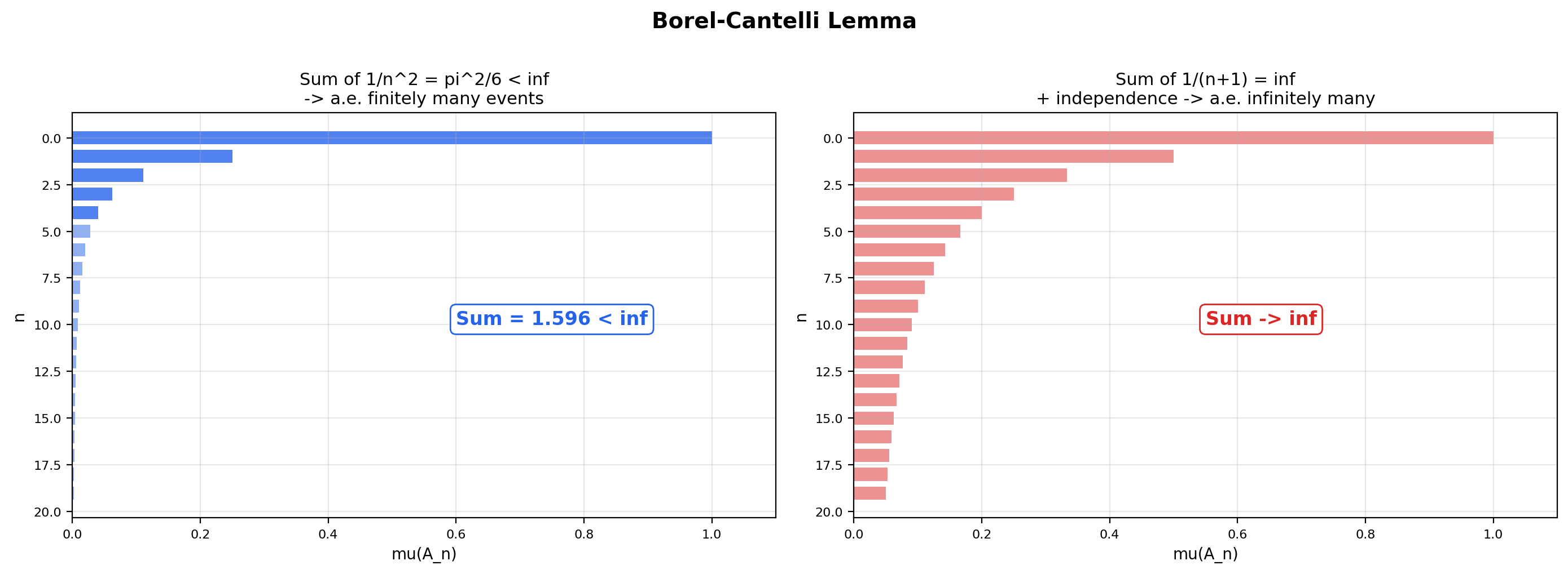
The next theorem is the workhorse for “with probability 1” statements in convergence theory. It’s a series convergence test recast as a measure-theoretic statement about tail events — the bridge between Topic 18 (Series Convergence & Tests) and probability theory.
🔷 Theorem 7 (Borel-Cantelli lemma (first form))
Let be a measure space and let be a sequence of measurable sets with
Then -almost every belongs to only finitely many of the . Formally,
Proof.
Let . The set is the collection of that belong to for infinitely many indices — every is in some for arbitrarily large . We must show .
For every , the definition of as an intersection gives
By monotonicity (Theorem 1.1) and countable subadditivity (Theorem 1.2),
The right-hand side is the tail of the convergent series . Since the full series converges, its tails tend to zero:
So . Combined with , we get .
The second form (which we will use without proof) reverses the implication when independence is assumed: if the are mutually independent and , then — almost every belongs to infinitely many of the . Together, the two forms give a complete dichotomy for tail events: either and a.e. point is in finitely many sets, or (under independence) and a.e. point is in infinitely many sets. This is the foundation for nearly every “with probability 1” theorem in the theory of stochastic processes and ML convergence.
📝 Example 17 (Empirical measure convergence — Glivenko-Cantelli)
Sample i.i.d. from the standard normal distribution. The empirical CDF is
This is the cumulative distribution function of the empirical measure . As grows, converges to the true CDF pointwise (by the law of large numbers) and in fact uniformly in (by the Glivenko-Cantelli theorem):
The Kolmogorov-Smirnov distance shrinks like , with the precise distributional behavior given by the Kolmogorov distribution. This is the rigorous statement that “training data converges to the true distribution as the sample size grows” — every empirical-risk-minimization argument in supervised learning depends on it.
13. Closing Reflection — Opening the Measure & Integration Track
This is the first topic in Track 7 — Measure & Integration — and the first advanced topic in formalCalculus. It builds the framework that the next three topics in the track will populate: the Lebesgue integral is built from simple functions and measures defined here; spaces are equivalence classes of measurable functions identified up to a.e.-equality; the Radon-Nikodym theorem characterizes when one measure has a density with respect to another. Without the sigma-algebra and measure framework constructed in this topic, none of the next three topics has a foundation to stand on.
The topic is also a bridge from classical calculus to modern probability. The measure-theoretic vocabulary built here — sigma-algebras as families of events, measures as probability assignments, measurable functions as random variables, “almost everywhere” as “with probability 1” — is exactly the vocabulary of probability theory. Every theorem in measure-theoretic probability starts from a measure space.
Connections & Further Reading
Prerequisites — topics you need first
Completeness & Compactness
Completeness of ℝ powers the closure-under-countable-operations arguments that define sigma-algebras. The Cantor set's compactness and the uncountability of ℝ from Topic 3 are reused throughout this topic.
The Riemann Integral & FTC
The Riemann integral's limitations — and the explicit failure on the Dirichlet function — are the entry point for the entire measure-theoretic story. Riemann-integrable functions are a strict subclass of Lebesgue-integrable functions.
Series Convergence & Tests
Countable additivity is defined via convergent series of measures, and the first Borel-Cantelli lemma is a series convergence test recast as a measure-theoretic statement about tail events.
Probability & The Union Bound
Where this leads — next in formalCalculus
The Lebesgue Integral
Builds the integral ∫ f dμ for non-negative measurable f as the supremum of integrals of approximating simple functions, then extends to general measurable functions. Proves the Monotone, Fatou, and Dominated Convergence theorems, plus Fubini-Tonelli for product measures.
Lp Spaces
Banach spaces of measurable functions where ‖f‖_p = (∫|f|^p dμ)^(1/p) < ∞. Equivalence classes under a.e.-equality use the null-set concept defined here as essential infrastructure.
Radon-Nikodym & Probability Densities
Characterizes when one measure ν has a density f = dν/dμ with respect to another measure μ. The bridge from measure theory to densities, conditional expectation, and Bayesian inference.
On to formalStatistics — where this calculus powers inference
Sample Spaces
A probability space (Ω, 𝓕, P) has 𝓕 a σ-algebra and P a probability measure on 𝓕. Kolmogorov's axioms are measure-theoretic. The Carathéodory extension theorem from this topic is the bedrock that makes every construction in formalStatistics rigorous.
Random Variables
A random variable X: Ω → ℝ is by definition a measurable function — X⁻¹(B) ∈ 𝓕 for every Borel set B. The σ-algebra σ(X) generated by X is the measurement resolution of X. Every event involving X is an element of σ(X).
Conditional Probability
Conditional expectation E[X|𝒢] is defined as the unique (a.s.) 𝒢-measurable random variable satisfying E[X·𝟙_A] = E[E[X|𝒢]·𝟙_A] for all A ∈ 𝒢. This is a σ-algebra-level construction — the Radon–Nikodym theorem guarantees its existence.
Modes Of Convergence
Almost-sure convergence P(X_n → X) = 1 is a statement about a measurable event in the σ-algebra. Convergence in probability, L^p convergence, and convergence in distribution are all measure-theoretic reformulations that reduce to the σ-algebra framework.
On to formalML — where this calculus powers ML
Gradient Descent
The set of initial conditions that converge to saddle points has Lebesgue measure zero — 'gradient descent avoids saddle points with probability 1' (Lee–Simchowitz–Jordan–Recht, 2016) is a measure-theoretic statement at base.
Semiparametric Inference
The conditional-expectation machinery used throughout — $\mathbb{E}[Y \mid X]$ as the $L^2(P)$ projection onto the $X$-measurable subspace, MAR's $Y \perp R \mid X$ conditional-independence statement, the EIF's pathwise-derivative computations against conditionally-centered scores — requires the $\sigma$-algebra foundations developed in this prereq.
Normalizing Flows
Normalizing flows are pushforward measures: T*μ_X = μ_Y. The change-of-variables formula for densities is a Radon-Nikodym derivative of the pushforward.
Concentration Inequalities
Markov, Chebyshev, Hoeffding — all are bounds on the measure of tail sets P(|X - μ| > t).
Extreme Value Theory
Extreme value theory's §§2–3 weak-convergence framework — convergence in distribution as weak convergence of probability measures, the Portmanteau theorem (Khintchine / type-convergence proof of §2.3), and Slutsky's theorem (throughout §3) — sits in the measure-theoretic substrate developed here.
References
- book Royden, H. L. & Fitzpatrick, P. M. (2010). Real Analysis Fourth edition. Chapters 2–3 cover sigma-algebras, Lebesgue measure, and Carathéodory's extension theorem with the same proof structure used here.
- book Folland, G. B. (1999). Real Analysis: Modern Techniques and Their Applications Second edition. Chapters 1–2 are the standard graduate-level reference for measure-theoretic foundations. The Vitali construction proof in Section 8 follows Folland's presentation.
- book Rudin (1976). Principles of Mathematical Analysis Chapter 11 — Lebesgue theory overview. Connects the real analysis foundations from earlier tracks to the measure-theoretic viewpoint
- book Rudin (1987). Real and Complex Analysis Chapters 1–2 — abstract measure construction and integration. The condensed, elegant treatment
- book Tao, T. (2011). An Introduction to Measure Theory Free PDF, excellent for self-study. Chapters 1–2 cover Lebesgue measure constructively with extensive geometric intuition.
- book Halmos (1974). Measure Theory The classic — rings, sigma-rings, extension theorems. Historically important and still widely referenced
- book Billingsley, P. (1995). Probability and Measure Third edition. Chapter 1 connects measure theory directly to probability — the bridge to formalml.com that this topic builds toward.
- book Durrett (2019). Probability: Theory and Examples Chapter 1 — measure theory for probabilists. Free online. Directly connects sigma-algebras to ML probability foundations