Lp Spaces
Function spaces with norms — from Hölder and Minkowski inequalities through Riesz-Fischer completeness to the geometric engine of regression, regularization, and modern function-space learning.
Abstract. Lp spaces are where functions become geometry. The Lebesgue integral from Topic 26 lets us integrate individual functions; Lp spaces organize those functions into vector spaces with norms, turning questions about function approximation into questions about distances and projections. We define the Lp norm, prove the three fundamental inequalities (Jensen, Hölder, Minkowski), and then prove the Riesz-Fischer theorem: Lp is complete, meaning every Cauchy sequence converges — using the Dominated Convergence Theorem from Topic 26 as the key tool. Completeness is what makes Lp spaces Banach spaces, and L2 a Hilbert space. The geometry of the Lp unit ball — diamond at p=1, circle at p=2, square at p=∞ — directly explains why L1 regularization produces sparsity and L2 regularization produces smoothness. Least-squares regression is an L2 projection. Fourier neural operators live in L2. Score matching minimizes an L2 distance between log-density gradients. This topic builds the function-space geometry that machine learning assumes you already have.
1. Three Puzzles Spaces Solve
Topic 26 built the Lebesgue integral and proved the three convergence theorems — Monotone Convergence, Fatou, and Dominated Convergence. We can now integrate measurable functions, take limits of integrals, and swap limits and integrals under modest hypotheses. That is enough to evaluate integrals, but it is not yet enough to organize them. The functions we integrate live as scattered objects: each one has its own integral, but we have no way to talk about how close two functions are, no way to talk about a sequence of functions converging to another function in a useful sense, and no way to do the kind of geometric reasoning — distances, projections, perpendicularity — that we routinely do with vectors in .
This topic fixes that. We organize measurable functions into vector spaces — the spaces — equipped with norms that turn function-space questions into geometric ones. Three puzzles motivate the construction.
1. When does least-squares regression have a unique solution? Linear regression finds the function in some class that minimizes . This is a “closest point” problem: we want the element of that is nearest to the data . But “nearest” requires a distance on functions. And for the minimization to have a solution at all, we need the space to be complete — minimizing sequences should converge to something inside the space, not slip out the side. We will see in Sections 6 and 7 that provides exactly this: a distance () and a completeness theorem (Riesz–Fischer) that guarantees minimizing sequences land somewhere legal.
2. Why do Fourier series converge “in energy” but not pointwise? Topic 22 showed that the partial Fourier sums of a discontinuous function — say, a square wave — overshoot at the discontinuity by about 9% no matter how many terms we add. This is the Gibbs phenomenon, and it tells us the partial sums do not converge pointwise to the target at the jump. Yet the integrated squared error goes to zero. So in some sense the partial sums do converge — just not pointwise. The right notion of convergence is convergence in the norm, which measures “how much energy is in the error” rather than “how big is the error at each point.” The two notions are different, and the difference is exactly the difference between asking “how does behave at ?” and “how does behave on average?”
3. What does it mean for two probability densities to be “close”? Generative models in machine learning are trained by minimizing some kind of distance between the learned density and the data density . But “distance between densities” is not a single thing — it depends on which norm we use to measure it. The distance is the total variation: it cares about every region where the two densities disagree. The distance penalizes large pointwise errors quadratically, smoothing out the influence of small errors and amplifying the influence of large ones. The distance demands uniform agreement: even one point of large disagreement makes the distance large. The choice of encodes a modeling decision about which kinds of errors we are willing to tolerate.
These three puzzles all reduce to the same demand: we need a vector space of functions, equipped with a norm, in which we can do geometric reasoning. That is what provides.
2. The Norm and Spaces
We start with the definition of the norm and then quotient by an equivalence relation to make it a true norm rather than a seminorm. The construction is one of the cleanest examples of “promote a seminorm to a norm by killing the kernel” in analysis.
📐 Definition 1 (The $L^p$ seminorm)
Let be a measure space, , and a measurable function . The seminorm of is
This is a seminorm, not a norm: , scalar multiplication pulls through (), and the triangle inequality holds (Minkowski, Section 5). What it does not satisfy is the definiteness axiom: does not imply — only almost everywhere.
The failure of definiteness is the whole reason we need the next step. If on a set of full measure but is non-zero on a measure-zero set, the integral and so — yet is not the zero function. To get a true norm we have to identify functions that agree almost everywhere.
📐 Definition 2 (The space $L^p(\mu)$)
Define the equivalence relation on measurable functions by
The space is the set of equivalence classes of measurable functions for which . On , the seminorm becomes a norm:
because now means ” a.e.”, which is exactly the statement that is the zero equivalence class.
The quotient is not just a technicality. Without it, we would have a seminormed space: a vector space where some non-zero elements have zero “length.” Quotient by the kernel (the functions of seminorm zero) and the seminorm becomes a norm. The norm is what gives us a metric (), and the metric is what gives us geometry — open balls, convergence, completeness, projections. From now on we will write when we mean the equivalence class .
The case needs its own definition because the formula has no obvious meaning when is infinite. The right notion is the essential supremum: the smallest constant that bounds except possibly on a null set.
📐 Definition 3 (The essential supremum and $L^\infty(\mu)$)
For a measurable function , the essential supremum is
The space consists of equivalence classes (under a.e.-equality) of measurable functions for which . Its norm is
The essential supremum is the natural measure-theoretic version of the supremum: it ignores what happens on null sets. A function that equals everywhere except at a single point where it equals has essential supremum , even though its actual supremum is — because the offending point is a null set, and a.e.-equivalence renders it invisible.
📝 Example 1 ($x^{-1/3}$ is in $L^p$ for $p < 3$ but not $L^3$)
Consider on with Lebesgue measure. We compute
So for every , with growing as approaches . At the integral diverges logarithmically and the norm becomes infinite, so . The number is called the critical exponent for this function: for any below it the function is integrable to the -th power, and for any at or above it, it is not. Different functions have different critical exponents, and that variability is what makes the family of spaces interesting — the same function can be a member of one space and not another.
📝 Example 2 (A function in every finite $L^p$ but not in $L^\infty$)
Let on extended by zero outside. As , , so — the function is bounded near . But near from below, , so approaches a finite positive value. The essential supremum is finite on most of the interval but blows up on the upper boundary in a different way:
So this particular is in fact in . To get a function in every finite but not in , take instead on : the integrals are all finite (the logarithm grows slower than any power, so integrating against it converges for every ), but as , so and . The membership patterns of as varies are surprisingly subtle, and they reflect different ways a function can fail to be “small.”
💡 Remark 1 (Notation: $f$ and $[f]$)
We will write throughout this topic when we technically mean . The abuse is universal in analysis and rarely causes confusion: when a statement holds for , it holds for every representative of , since the statements are themselves only sensitive to a.e.-behavior. Two functions in the same equivalence class are interchangeable for every purpose we care about — integrals against them, norms, convergence in — so working with representatives instead of classes is harmless and notationally cleaner.
💡 Remark 2 (Why the quotient is essential)
The quotient by a.e.-equivalence is not optional. Without it, the seminorm is not a norm, the functional does not separate points, and the metric is not a metric — two distinct functions can be at distance zero. None of the geometric constructions we want — open balls, convergence in norm, completeness, orthogonal projection — make sense in a seminormed space, because the topology is not Hausdorff. The quotient promotes the seminorm to a norm by collapsing every equivalence class to a single point, and that single move makes the entire theory of spaces possible.
The interactive viz below makes the dependence of on concrete: pick a function from the dropdown, slide , and watch how the integrand redistributes mass as changes. For large the mass concentrates where is largest, and the norm approaches the essential supremum.
A smooth half-cycle of a sine wave on [0, 1]. As p grows, |f|^p concentrates where |f| is largest — for large p the integrand is dominated by the peak, and ||f||_p approaches the essential supremum (||f||_∞).
3. Jensen’s Inequality
Before we prove Hölder and Minkowski, we need one preparatory inequality that is interesting in its own right and that also previews the proof technique. Jensen’s inequality says that integrating a convex function against a probability measure gives at least the convex function applied to the integral. It is the single inequality that connects measure theory to information theory: every non-negativity result about KL divergence, mutual information, and entropy is a Jensen application.
🔷 Theorem 1 (Jensen's inequality)
Let be a probability space (), let , and let be convex. Then
Proof.
The proof uses one fact about convex functions: at every point, a convex function has a supporting line. That is, for every there exists a slope (the right or left derivative of at , or any value in between if is not differentiable at ) such that
This is the definition of being convex, restated geometrically: the graph of lies above every one of its tangent lines.
Step 1: Choose . Set — the integral of against . Since is a probability measure and , this integral is a finite real number. Choose any supporting line of at with slope .
Step 2: Apply the supporting-line inequality pointwise. For each we have , so the supporting-line inequality with gives
This holds at every point , with the same constants and .
Step 3: Integrate against . Both sides of the pointwise inequality are measurable functions of , and the right-hand side is integrable because it is an affine function of and . Integrating preserves the inequality:
The right side splits using linearity of the integral:
We used (probability measure) for the first term and for the second. Substituting on the right gives the conclusion.
The proof is short but geometrically sharp: convexity says the graph of lies above its tangent line, and integration is linear, so anything you can say about a tangent line you can say about its integral. Jensen’s inequality is, in essence, the statement that integration commutes with affine transformations and convex functions only “lose” information in the right direction.
📝 Example 3 (KL divergence is non-negative — the first Jensen application)
Let and be probability measures on with (i.e., is absolutely continuous with respect to — every -null set is -null), and let be the Radon–Nikodym density (we will formalize Radon–Nikodym in Topic 28; for now treat as the “ratio” of to ). The Kullback–Leibler divergence of from is
The function is convex on . Apply Jensen’s inequality to against the probability measure :
Now compute the integral on the left. Since , we have . So , and we get
with equality iff is constant -a.e. (the equality case of Jensen for strictly convex ), which means is constant, which means a.e., which means . This is Gibbs’ inequality, the foundational non-negativity result of information theory.
💡 Remark 3 (Jensen connects measure theory to information theory)
Jensen’s inequality is the bridge from measure theory to information theory, and it is the only bridge most people remember after they leave grad school. Every non-negativity statement in information theory — Gibbs’ inequality (KL ), the chain rule for KL divergence, the data processing inequality, the convexity of mutual information — is a Jensen application. Variational methods in machine learning rest on the same foundation: the ELBO (evidence lower bound) used in variational autoencoders and Bayesian neural networks is Jensen applied to , and the inequality slack is exactly the KL divergence between the variational posterior and the true posterior. Forward link: Variational Inference.
4. Hölder’s Inequality
Hölder’s inequality is the central duality inequality of spaces. It says that the integral of a product of two functions is bounded by the product of their respective norms — provided the exponents are conjugate. The notion of conjugate exponents is the engine of the entire duality theory we will develop in Section 10.
We prove Hölder via Young’s inequality, which is itself a one-line consequence of the convexity of the exponential. Young’s inequality is the pointwise inequality that, when integrated, becomes Hölder.
🔷 Proposition 1 (Young's inequality)
For and conjugate exponents satisfying :
Equality holds iff .
Proof.
The cases or are trivial, so assume .
Step 1: Rewrite the product as an exponential. Take logarithms inside an exponential:
The exponent on the right is a convex combination of and , with weights and that sum to by the conjugacy condition.
Step 2: Apply convexity of the exponential. The function is convex. For any convex combination with and , convexity gives . With , , , and :
Step 3: Simplify. Note that and . Combining the previous two displays:
Equality in the convexity step requires (the two points being averaged are the same), which after exponentiation is .
Young’s inequality is a pointwise statement: it bounds the product of two non-negative numbers by an explicit sum involving their powers. Hölder’s inequality is what you get by integrating Young pointwise after a clever normalization step — it converts a pointwise bound on numbers into an integrated bound on functions.
🔷 Theorem 2 (Hölder's inequality)
Let and with and (with the convention , so pairs with and vice versa). Then and
Proof.
We prove the case (so as well). The endpoint cases and are immediate from the definition of as the essential supremum: a.e., so .
Step 1: Trivial cases. If , then a.e., so a.e., and both sides of the inequality are zero. Similarly for . So we may assume and .
Step 2: Normalize. Define the rescaled functions
By construction and . Proving for the normalized pair will give after multiplying through by .
Step 3: Apply Young’s inequality pointwise. For each , set and in Young’s inequality:
This holds at every point , with the same and .
Step 4: Integrate against . Both sides are measurable functions of , and the right-hand side is integrable since and . Integration preserves the inequality:
By construction, , and likewise . The right side becomes , so
Step 5: Un-normalize. Multiplying both sides by :
The proof is a perfect example of the “integrate a pointwise inequality” technique. Young’s inequality is a pointwise bound on numbers; integrating it after a normalization step turns it into an integrated bound on functions. The conjugacy condition is what makes the right-hand side simplify to — without it, the proof would not close.
📝 Example 4 (Cauchy–Schwarz is Hölder at $p = q = 2$)
The most familiar special case of Hölder is the Cauchy–Schwarz inequality:
This is Hölder’s inequality with — and the conjugacy condition checks out. Cauchy–Schwarz is the inequality that makes an inner product space: if we define , then Cauchy–Schwarz says , which is the defining property of an inner product. Section 9 develops this perspective in detail.
📝 Example 5 (Hölder with explicit power functions)
Consider and on with Lebesgue measure, and (note ). Compute each piece of Hölder:
The product , so Hölder gives
The inequality holds with a ratio of about — close to equality but not sharp. The interactive viz below lets you slide and watch this ratio evolve, including for choices that drive the ratio toward (the Young’s-inequality saturation case).
A sine half-cycle and a quadratic — Hölder is strict and the ratio sits well below 1. The bar chart on the right compares the two sides of the inequality. Slide p (or toggle Minkowski) to see how the ratio responds.
💡 Remark 4 (When does Hölder hold with equality?)
Tracing through the proof, equality in Hölder is equivalent to equality in the Young’s-inequality step at -almost every point, which (Proposition 1) requires almost everywhere. Un-normalizing, this becomes: there exist constants , not both zero, such that a.e. Functions of this form — where and are proportional — are called conjugate pairs.
The sharpness condition is surprisingly fragile: it is not enough for and to “look similar.” Consider and on with , (the “power-pair” preset in the explorer above). The powers look naturally matched, but the pointwise check fails: while , so and differ by a factor of — they are not proportional, and the Hölder ratio sits at about rather than .
To actually get equality at , , we need . The simplest way: take and with , so , so . Choosing gives , and now exactly. This is the “power-pair-sharp” preset in the explorer — flip to it and the ratio snaps to to within quadrature precision. Sharp Hölder pairs are the analogue of eigenvalue–eigenvector pairs in a finite-dimensional inner product space: they expose the “tightness directions” of the inequality.
5. Minkowski’s Inequality
Minkowski’s inequality is the triangle inequality for . It is the inequality that promotes from a “size functional” to a norm: the triangle inequality is exactly the missing axiom that the seminorm definition didn’t give us for free. We prove Minkowski directly from Hölder.
🔷 Theorem 3 (Minkowski's inequality)
Let with . Then and
Proof.
The cases and are immediate: pointwise, and integrating (for ) or taking the essential supremum (for ) gives the result. We prove the case via Hölder.
Step 1: Bound in terms of and . The triangle inequality for absolute values gives pointwise, so
Distributing:
Step 2: Integrate. Integrating both sides against :
Step 3: Apply Hölder to each term. Let be the conjugate exponent of , so . Apply Hölder’s inequality to the first integral with in the slot and in the slot:
Compute . So the right side is . Similarly for the second integral:
Step 4: Combine and divide. Substituting back into Step 2:
If the inequality holds trivially; otherwise we may divide both sides by . Note that by conjugacy, so . The result is
The trick in the proof is “split as and apply Hölder,” where the conjugate exponent is engineered exactly so that — the inner integrals collapse back to , which we can then divide out. This is a small algebraic miracle that only works because of the conjugacy condition.
📝 Example 6 (Minkowski with disjoint indicators)
Take and on with Lebesgue measure, and . Compute the three quantities:
(The supports are disjoint, so is the indicator of — except possibly at the single point , which has measure zero.) Minkowski says , which here becomes
This is a strict inequality with a healthy gap — about slack. The reason: in the norm, “disjoint supports” is not the same as “orthogonal.” The two functions overlap at exactly one point (a measure-zero set), but the geometry treats them as if they were in different “directions” yet still adds them in a non-orthogonal way. The disjoint indicators are orthogonal in the inner-product sense (, by Section 9), and for orthogonal vectors the Pythagorean identity says , which is . So the Minkowski inequality holds with strict inequality, but the Pythagorean identity holds with equality — these are two different statements about the same pair, and they are both true.
💡 Remark 5 ($p < 1$: the triangle inequality fails)
The Minkowski proof uses the fact that is convex on , which holds for . For the function is concave, and the triangle inequality reverses direction. Concretely, with the same disjoint indicators and but :
Comparing: but . So — the “norm” of the sum is larger than the sum of the “norms.” The triangle inequality fails, is not a norm, and is not a normed space. (It is still a topological vector space; the formula defines a translation-invariant metric. But there is no norm.) For this reason the entire theory in the rest of this topic restricts to .
6. Is a Normed Vector Space
We have all the pieces. Sections 2 and 5 give us the seminorm, the quotient that promotes it to a norm, and the triangle inequality. Putting them together:
🔷 Theorem 4 ($L^p(\mu)$ is a normed vector space)
For every , is a normed vector space. That is:
The first axiom (definiteness) is the part where the a.e.-quotient earns its keep: implies , which implies a.e., which implies a.e., which is exactly the statement that in (as an equivalence class). The second axiom (homogeneity) is immediate from pulling the constant out of the integral. The third axiom (triangle inequality) is Minkowski. So is a normed vector space.
But “normed vector space” is not yet enough for the geometric reasoning we want. Real geometry — the kind where minimizing sequences converge, where projections exist, where Cauchy implies convergent — needs completeness. That is what Section 7 establishes: is not just a normed vector space, it is a Banach space (a complete normed vector space). The Riesz–Fischer theorem is the cornerstone result of this topic, and its proof uses the Dominated Convergence Theorem from Topic 26 in an essential way.
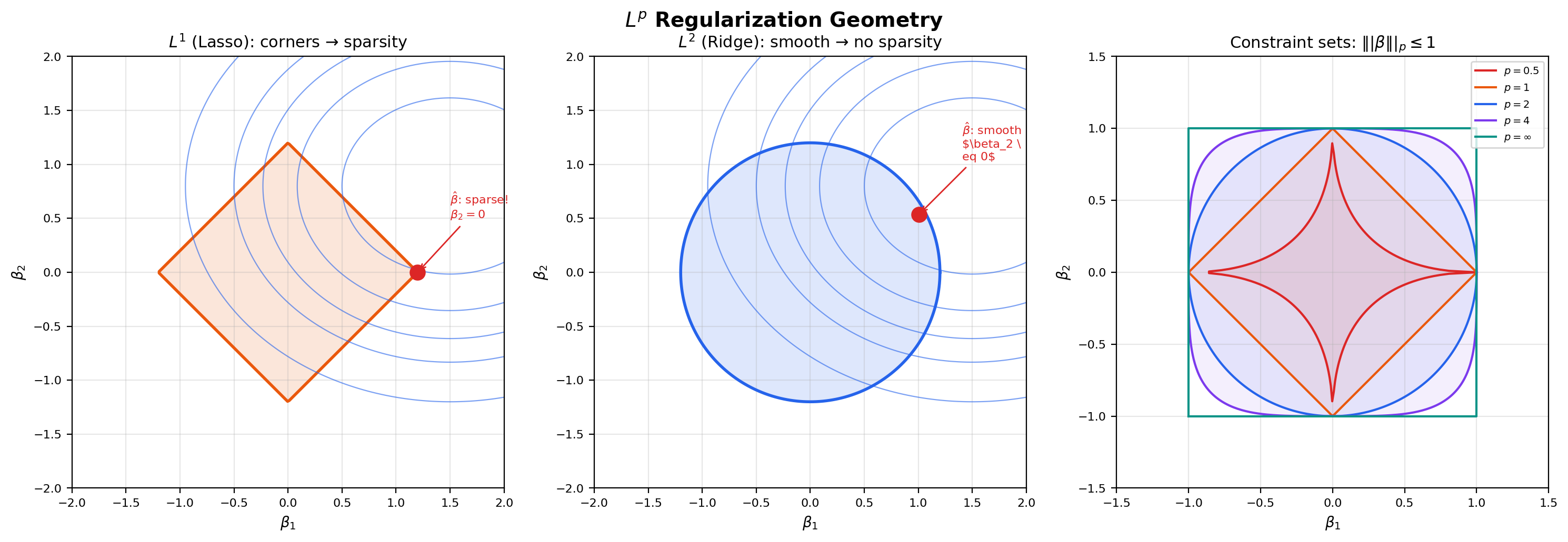
Before we get there, let us look at what these norms actually mean geometrically. The unit ball of an norm — the set of vectors with norm at most — is a shape that depends in a striking way on . At the ball is a diamond (or, in higher dimensions, a cross-polytope); at it is a sphere; at it is a cube. The shape morphs continuously between these extremes as varies, and the morphing is the visual core of the entire theory of regularization in machine learning. The flagship explorer below lets you slide and watch the unit ball change shape — pay particular attention to the corners that appear at and disappear at , because those corners are exactly the geometric reason that regularization (Lasso) produces sparse solutions and regularization (Ridge) does not.
Slide p from 0.5 to 20 (or toggle p = ∞) to watch the unit ball morph from a non-convex star (p < 1) through a diamond (p = 1), to a circle (p = 2), to a square (p = ∞). The corners at p = 1 are exactly why L¹ regularization (Lasso) produces sparse solutions.
💡 Remark 6 (The quotient promotes a seminorm to a norm)
Looking back at the construction: the seminorm on the space of measurable functions has a non-trivial kernel — the set of functions with — and that kernel is precisely the set of functions that are zero almost everywhere. Quotienting by the kernel collapses the kernel to a single point (the zero element), and on the quotient the seminorm becomes a norm. This is a general construction: in any seminormed vector space, the kernel of the seminorm is a linear subspace, and the quotient by the kernel is automatically a normed space. is one of the most famous applications of this general fact, and it is the reason measure-theoretic functional analysis can use the geometric language of normed vector spaces at all.
7. Completeness — The Riesz–Fischer Theorem
The single most important fact about spaces — the result that makes essentially every downstream use of work — is that is complete. Every Cauchy sequence converges to an element of the space. This is not automatic for normed vector spaces in general (the space of polynomials with the norm, for example, is not complete: a Cauchy sequence of polynomials can converge to a non-polynomial), and it is not at all obvious from the definition. The Riesz–Fischer theorem is the proof.
📐 Definition 4 (Cauchy sequence in $L^p$)
A sequence in is Cauchy if for every there exists such that for all .
Equivalently, as .
The Cauchy condition is purely internal to the sequence — it asks “are the terms getting closer to each other?” without ever mentioning a candidate limit. Completeness is the assertion that every Cauchy sequence in fact has a limit in the space. The Riesz–Fischer theorem says has this property.
🔷 Theorem 5 (Riesz–Fischer theorem)
For every and every measure space , the space is complete: every Cauchy sequence in converges to an element of .
In particular, with the norm is a Banach space.
Proof.
We prove the case . The case is a separate (easier) argument that we sketch in Remark 7. Let be a Cauchy sequence in . We will construct a candidate limit, show that a subsequence converges to it, and then use the Cauchy property to upgrade subsequence convergence to full-sequence convergence.
Step 1: Extract a fast-converging subsequence. Since is Cauchy, we can choose indices such that
This is possible because the Cauchy condition with gives an index such that for ; we just choose .
Step 2: Bound the partial-sum-of-differences. Define the non-negative function
Each is measurable and non-negative. By Minkowski’s inequality applied times,
So the norms of the partial sums are uniformly bounded by .
Step 3: Pass to the monotone limit. The sequence is monotone increasing — adding another non-negative term cannot decrease the sum. By the Monotone Convergence Theorem (Topic 26, Section 5) applied to , the pointwise limit
exists in at every and satisfies
So , and in particular for -almost every . This is the key consequence of the bound: the infinite sum of absolute differences is finite a.e.
Step 4: Construct the candidate limit . Where — i.e., on a set of full measure — the series
is absolutely convergent. (This is the standard “absolute convergence implies convergence” fact for real-valued series, applied at each .) The partial sums of this series are exactly — the series telescopes — so we define
and on the null set where the series fails to converge. The function is measurable (as the a.e.-limit of measurable functions, redefined on a null set).
Step 5: . We need to check that the candidate limit actually lives in . The triangle inequality gives, for every ,
Letting and using the pointwise limit definition of :
So a.e., and both and , so by Minkowski.
Step 6: in . We use the Dominated Convergence Theorem from Topic 26. Define . We need:
(a) a.e. as . This holds because a.e. by Step 4 and is continuous.
(b) A dominating function. By the same triangle-inequality argument as Step 5, for almost every (cap it through and ). So
The function is in because from Step 3. So is dominated by an integrable function for every .
DCT now gives , which is exactly . So in along the chosen subsequence.
Step 7: The full sequence converges. We have shown that the subsequence converges to in . To upgrade this to convergence of the full sequence , fix . Since is Cauchy, choose such that whenever . Since in , choose such that and . Then for any ,
So and the full sequence converges to in .
The proof has the unmistakable structure of a “real analysis lower-bound transfer” argument: extract a fast-decaying subsequence so that the differences are summable, sum the differences to get an a.e. limit, dominate to get convergence, then use Cauchyness to extend from subsequence to full sequence. The DCT plays the role of the closer — once we have an a.e. limit and a uniform dominator, DCT does the rest. Everything else in the proof is preparatory work to set up the DCT application.
📝 Example 7 (A Cauchy sequence converging in $L^2$)
The smooth-step functions defined by
are smooth approximations to the indicator . As grows the two transitions sharpen, and pointwise on the interior and at every interior point of — so the convergence is pointwise everywhere except at the two boundary points , which are a null set.
Numerically, decays rapidly: at it is around , at around , at around . The sequence is Cauchy in — for any both large, the two functions both approximate the indicator and so are close to each other — and Riesz–Fischer guarantees a limit in . That limit is the equivalence class . The interactive viz below lets you advance and watch both the function and the -norm difference.
Smooth tanh-mollified approximations to 1_[0, 1]. As n grows the transitions sharpen and f_n converges to the indicator in every L^p (1 ≤ p < ∞). The bar chart shows how the L^p norm difference decays as k grows — completeness of L^p (Riesz–Fischer) guarantees that this Cauchy sequence converges in the L^p norm to the limit shown.
💡 Remark 7 (Why completeness matters for ML — and the $p = \infty$ case)
Completeness is the abstract guarantee that minimizing sequences in optimization actually converge to something legitimate. In gradient descent, EM, variational inference, and any other iterative procedure that produces a sequence of approximations to a target, completeness of the ambient space is what guarantees that “Cauchy” implies “converges to a real function.” Without completeness, a perfectly well-behaved minimizing sequence could “escape” the space and converge to something pathological — a delta function, a non-measurable beast, or nothing at all. Forward link: Gradient Descent.
The case is technically separate but easier than the proof we just gave. If is Cauchy in , then for every there is an such that for -almost every when . Taking a countable union of null sets (one per pair ) and removing it from leaves a set on which is uniformly Cauchy as a sequence of bounded functions, so it converges uniformly to a bounded function . Then . So is also complete.
8. Density Results
The space has many “nice” subspaces — simple functions, continuous compactly supported functions, polynomials on compact intervals, smooth functions — and an important question is whether these subspaces are dense. Density means: every function can be approximated arbitrarily well in the norm by an element of the subspace. Density results are the bread and butter of approximation theory: they say that questions about general functions can often be reduced to questions about simpler, more tractable functions.
🔷 Theorem 6 (Density of simple functions in $L^p$)
For every , the simple functions in are dense: for every , there exists a sequence of simple functions with .
Proof.
By Topic 25’s simple-function approximation theorem, there exists a sequence of simple functions with pointwise and pointwise (and even uniformly on sets where is bounded, but we only need pointwise here).
The sequence converges pointwise to zero. To upgrade pointwise convergence to convergence, we need a dominator. The triangle inequality gives
The function is in because , so . By the Dominated Convergence Theorem (Topic 26),
Taking -th roots gives .
The proof is a beautiful one-line application of DCT: we already know the simple functions converge pointwise from Topic 25, and we already know is integrable from , so DCT gives the rest. This is the recurring pattern of this topic: every density and convergence result is “find a pointwise limit, find a dominator, apply DCT.”
For on with Lebesgue measure there is an even stronger density result: continuous, compactly supported functions are dense. This is what justifies using neural networks — universal approximators of continuous functions — to approximate functions.
🔷 Theorem 7 (Density of $C_c(\mathbb{R}^n)$ in $L^p(\mathbb{R}^n)$)
For , the space of continuous, compactly supported functions is dense in : for every , there exists a sequence with .
Proof.
The proof has two stages. First, we approximate by simple functions (Theorem 6). Second, we approximate each simple function by a continuous compactly supported function via mollification.
A simple function on is a finite linear combination of indicator functions of measurable sets. By inner regularity of Lebesgue measure, every measurable set of finite measure can be approximated from inside by a closed set (and outside by an open set) up to arbitrarily small measure. Urysohn’s lemma then gives a continuous function that is on the closed set, outside the open set, and varies linearly in between. Taking the linear combination with the same coefficients as the simple function, we obtain a continuous compactly supported function that differs from the simple function in norm by an arbitrarily small amount. Iterating both approximation steps with errors at the -th step and applying the triangle inequality completes the proof.
A full version of this argument lives in Folland §6.1 (or Brezis §4.1 for the case in detail). The key technical lemma is mollification: convolving an function with a smooth, compactly supported “bump” function (a mollifier) produces a smooth approximation that converges in as the mollifier scale shrinks.
📝 Example 8 (Density failure in $L^\infty$)
The density of in holds for , but fails at . Consider as an element of , and let be any continuous function. Near , must transition continuously from to — there is no “jump.” So cannot equal for and for simultaneously: at any , there will be points where or points where . The same argument applies near .
Quantitatively: for any continuous , the difference has . (In a neighborhood of either jump, and differ by at least in essential supremum.) So is not dense in . The closure of in is the smaller space of continuous functions vanishing at infinity, which is a proper subspace. The density failure at is one of several reasons is “harder” than the other spaces and why most theorems in this topic explicitly restrict to .
💡 Remark 8 (Density for neural network approximation)
Density of in has a striking machine learning consequence. The universal approximation theorem (which we will state precisely in Approximation Theory — Topic 20) says that neural networks with one hidden layer can approximate any continuous function uniformly on compact sets. Combined with density of in , this gives:
Any function can be approximated arbitrarily well in norm by a neural network.
The logic is a two-step approximation: given , first find a continuous compactly supported with (Theorem 7), then find a neural network with (universal approximation), and conclude . This is the existence proof behind every “neural networks can approximate any function” claim in machine learning textbooks. What it leaves open — and what most of modern statistical learning theory addresses — is the question of how big the network has to be to achieve a given approximation error.
9. as a Hilbert Space (Preview)
Among all the spaces, is special. The norm comes from an inner product — a bilinear pairing that satisfies — which gives a richer geometric structure than the other spaces. In particular, has notions of orthogonality and projection that the other spaces lack. This section previews the inner-product structure; the full Hilbert space theory will be developed in Topic 31.
📐 Definition 5 (The $L^2$ inner product)
For real-valued , the inner product is
For complex-valued functions, the inner product uses the conjugate of : .
🔷 Proposition 2 (Inner product axioms on $L^2$)
The inner product is well-defined (the integral is finite by Cauchy–Schwarz; see Example 9), bilinear in the real case (sesquilinear in the complex case), symmetric (conjugate-symmetric in the complex case), and positive definite: with equality iff in . Moreover,
So the norm is the norm induced by the inner product, and is an inner product space. Combined with the Riesz–Fischer completeness from Section 7, this makes a Hilbert space: a complete inner product space.
📝 Example 9 (Cauchy–Schwarz as Hölder at $p = q = 2$)
For , the Cauchy–Schwarz inequality
is exactly Hölder’s inequality with . The first inequality is (the integral version of ), and the second is Hölder. So Cauchy–Schwarz is not an independent inequality — it is a special case of the more general Hölder result we proved in Section 4. This is the geometric reason that is the “best-behaved” space: at , the basic inequality of the inner-product structure coincides with the basic inequality of the integral structure.
📝 Example 10 (The Fourier basis is orthonormal in $L^2([0, 2\pi])$)
On the interval with normalized Lebesgue measure , the complex exponentials for form an orthonormal system: (Kronecker delta). To see this, compute
If , the integrand is and the integral is , so . If , the integral evaluates to (the function is -periodic). So the Fourier basis is orthonormal, which means partial Fourier series can be computed by a finite-dimensional projection, the Fourier coefficients are inner products , and Parseval’s identity is the Pythagorean theorem in the Hilbert space . Forward link: Fourier Series (Topic 22).
🔷 Proposition 3 (Orthogonal projection (statement only))
Let be a closed linear subspace. For every , there exists a unique element — the orthogonal projection of onto — that minimizes over all . The error vector is orthogonal to every element of :
A full proof requires the Hilbert space theory developed in Topic 31, but the statement is accessible now and is the central geometric fact about .
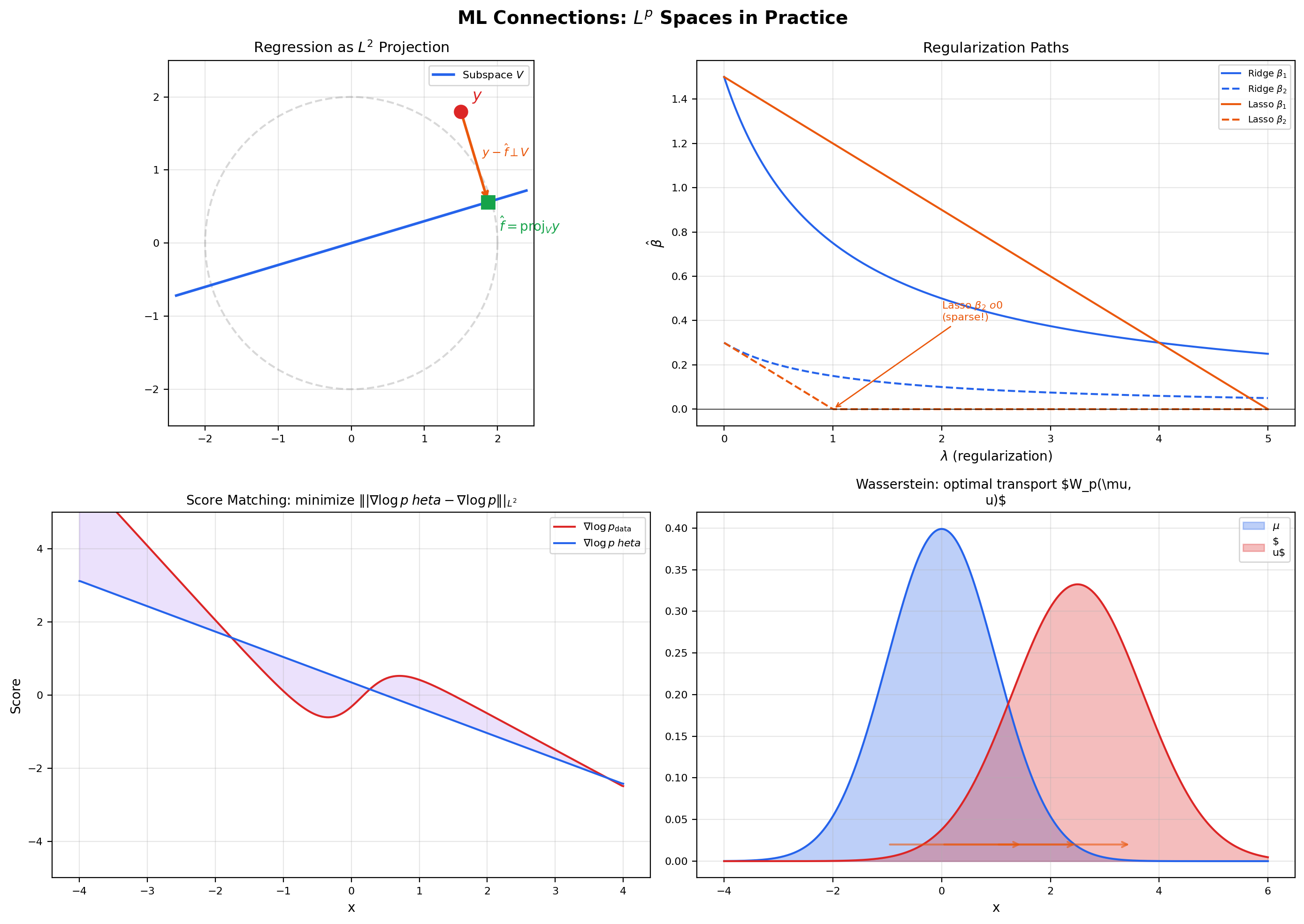
💡 Remark 9 (Regression as $L^2$ projection)
Linear regression is exactly an orthogonal projection in . Given data and a design matrix , the least-squares estimator is . The vector is the orthogonal projection of onto the column space of (a closed subspace of with counting measure), and the normal equations are the orthogonality condition for every — i.e., the residual is orthogonal to every linear combination of the columns of . This identification is not a metaphor: it is literally the same thing. Generalized least squares uses a weighted inner product for some positive-definite weight , and the geometry remains the same — projection onto the column space, orthogonality of the residual, existence and uniqueness via the projection theorem. Forward link: Regression.
10. Duality —
Every normed vector space has a dual space : the space of bounded linear functionals , with the operator norm . For spaces with conjugate exponents , the dual space has a particularly clean characterization — it is isometrically isomorphic to the other space in the conjugate pair. This is the Riesz representation theorem for , and it is the foundation of duality theory.
🔷 Theorem 8 (Riesz representation theorem for $L^p$)
Let and let be a -finite measure space. Let be the conjugate exponent of , so . Then every bounded linear functional has the form
and the operator norm of equals the norm of the representing function:
In particular, the map is an isometric isomorphism , often written as .
Proof.
We sketch the proof; full details are in Folland §6.2 or Royden §19.5.
Embedding . Given , define . By Hölder’s inequality, , so is a bounded linear functional with . To show equality, take ; a direct computation gives and , so . Combining, .
Surjectivity. Given a bounded linear functional , we want to find with . For each measurable set of finite measure, define . Linearity of on indicator functions makes a finitely additive set function; boundedness and a countable-additivity argument upgrade to a -additive signed measure. Moreover, if , then in , so . So is absolutely continuous with respect to (every -null set is -null).
By the Radon–Nikodym theorem, absolute continuity implies that has a density , so . By construction, for every set of finite measure. Linearity then extends this from indicators to simple functions, and density of simple functions in (Theorem 6) plus continuity of extends it to all of . So on all of . Showing uses the operator norm bound and a clever choice of test function similar to the embedding step.
💡 Remark 10 (Endpoint cases — $L^1$, $L^\infty$, and the asymmetry)
The same theorem holds at , — namely , with the same proof structure but using -finiteness explicitly to handle the unboundedness of representing functions. The mirror statement is false: the dual of is strictly larger than , containing “singular” functionals such as evaluation at a point that cannot be represented as for any . This asymmetry — duality is symmetric for but not at the endpoints — is one of the features that make the most idiosyncratic space and the reason most theorems in functional analysis explicitly exclude .
📝 Example 11 (Dual pairing in finite dimensions: $(\ell^p)^* = \ell^q$)
When with counting measure, becomes — the space of -tuples with the -norm . Hölder becomes the finite-dimensional inequality , and the Riesz representation theorem becomes the statement that every linear functional has the form for a unique , with . So the dual space of with the -norm is with the -norm. In coordinates, every linear functional is a dot product — but the norm on the dual is the -norm rather than the -norm. This is the finite-dimensional fingerprint of the general duality theorem, and it is the foundation of every constrained optimization argument that uses Lagrangian duality with -norm constraints.
11. Computational Notes
A few practical observations about computing norms in code, since machine learning practitioners encounter discrete and continuous norms constantly.
-
Discrete norms.
numpy.linalg.norm(x, ord=p)computes for a vector . This is against the counting measure on . Theord=np.infcase gives — the discrete essential supremum, which equals the actual supremum because every singleton has positive measure under counting measure. -
Continuous norms. For an analytic or sampled function,
scipy.integrate.quad(lambda x: abs(f(x))**p, a, b)[0]**(1/p)computes on via numerical quadrature. This is the “integrate , then take the -th root” recipe straight from Definition 1, and it works for any . For , replace with a sup over a fine grid. -
torch.nn.functional.mse_lossis a discrete computation. The mean squared error loss is , which is against the normalized counting measure on (assigning measure to each point). The factor of converts counting measure to the empirical measure, which is what makes MSE the natural loss for finite-sample expected value estimation. -
Regularization geometry: the ball is the constraint set. Ridge regression solves — the regularization term constrains to lie inside an ball, which is a sphere with no corners. The least-squares contour is generically tangent to the sphere at a point with all coordinates non-zero, so Ridge “shrinks” coefficients but never sets them exactly to zero. Lasso solves — the regularization constrains to an ball, which is a diamond with corners on the coordinate axes. The least-squares contour generically intersects the diamond at a corner, where one or more coordinates are exactly zero, so Lasso produces sparse solutions. Elastic net uses both penalties: , and its constraint set is a smooth blend of the two extremes. The flagship ball viz in Section 6 makes this geometric explanation visual.
📝 Example 12 (Numerical verification of Hölder)
For and on , , , computing each norm via scipy.integrate.quad:
Hölder bound: . The inequality holds with substantial slack (ratio about ). The ratio is far from because and are not proportional — the conjugacy condition for sharp Hölder fails. Compare to the power-pair example in Section 4 where the ratio approached because the functions were specifically designed to be a conjugate pair.
12. Connections to Machine Learning
spaces are not an abstract curiosity — they are the function-space framework that every modern ML algorithm implicitly assumes. Five concrete connections illustrate the range.
Regression as projection. Least-squares regression finds the closest element of a closed subspace of , and the existence-and-uniqueness of the minimizer is exactly the orthogonal-projection theorem from Section 9. The normal equations are the orthogonality condition. Generalized least squares uses a weighted norm where the weights encode observation precisions, and weighted regression remains a projection — just in a re-weighted Hilbert space. Forward link: Regression.
Regularization geometry. The shapes of the and unit balls determine the qualitative behavior of regularized estimators. The ball has corners on the coordinate axes; the intersection of a level curve of the data-fit term with a corner produces sparsity (some coordinates exactly zero). The ball is a smooth sphere; intersections never sit on axes, so regularization shrinks coordinates but never zeros them out. This is why Lasso selects features and Ridge does not — and the explanation is purely geometric, not statistical.
Fourier neural operators. Fourier neural operators (FNO) learn mappings between function spaces, typically . The training objective is an loss over function pairs from a PDE dataset: . Riesz–Fischer guarantees that the optimization happens in a complete function space — minimizing sequences converge inside . Without completeness, the optimization could “escape” to non-functions, and the entire approach would be ill-defined. Forward link: Fourier Neural Operators.
Score matching. Score matching trains a generative model by minimizing the distance between the score functions (gradients of log-densities) of the model and data: . The objective is well-defined precisely when both score functions live in . Denoising score matching, sliced score matching, and diffusion-model training are all computational tricks for evaluating this functional without knowing explicitly. Forward link: Score Matching.
Wasserstein distances and optimal transport. The Wasserstein- distance between two probability measures is
which has the structure of an norm in the space of couplings . The Kantorovich dual formulation uses the duality from Section 10: , where the supremum is over -Lipschitz functions (an subspace). The dual side replaces the infimum over couplings with a supremum over functions, and the duality is exactly / duality applied to the optimal transport setting. Forward link: Wasserstein Distances.
📝 Example 13 ($L^1$ vs. $L^2$ regularization paths)
Consider a 2D regression with parameter vector . As the regularization strength varies, the Ridge path moves smoothly from the OLS solution toward the origin , with both coordinates shrinking continuously and never reaching zero except in the limit. The Lasso path is piecewise linear and kinks at values of where one of the coordinates first becomes exactly zero. After the kink, the Lasso solution stays on the axis — it has selected one feature and dropped the other. The qualitative difference between “smooth shrinkage” (Ridge) and “kink-then-zero” (Lasso) is entirely a consequence of the ball geometry: the ball is differentiable, so the optimum moves smoothly; the ball has corners, so the optimum hits a corner at some and stays there.
📝 Example 14 ($L^2$ convergence of Fourier partial sums)
Take on . The partial Fourier sums exhibit the Gibbs phenomenon: at the discontinuities and , overshoots by about no matter how large is. So does not converge pointwise to at the jumps. But the error decays:
since the Fourier coefficients of are square-summable (Parseval’s identity). The decay is moderate — about — but it goes to zero. So in but not pointwise. The Gibbs overshoot is an artifact of pointwise behavior at a measure-zero set, and the norm is insensitive to it because it integrates against a measure that assigns no mass to individual points. This is the cleanest example of “two notions of convergence give different answers, and the answer that survives in the long run is the one that respects the underlying measure.”
13. Closing Reflection — From Functions to Function Spaces
This is the third topic in Track 7 — Measure & Integration — and the third advanced topic in formalCalculus. Topics 25 and 26 built the framework and the integral; this topic built the function spaces. The combination is the foundation that the next several topics across measure theory, functional analysis, and probability rest on. The Riesz–Fischer completeness theorem proved here is what makes everything downstream possible: without completeness of , there is no Banach space theory, no Hilbert space theory, no Radon–Nikodym theorem, no functional-analytic optimization. Topic 27 is the smallest topic that the rest of modern analysis depends on.
The central editorial pivot in this topic was from individual functions to spaces of functions. Topic 26 asked “does this function have a finite integral?” and Topic 27 asks “how far apart are these two functions?” Both questions are about measurable functions, but the second one requires organizing functions into a vector space with a norm — and that organization is exactly what makes function-space methods feel like linear algebra. Once is in place, the analogies between and function spaces (vectors / functions, dot products / integrals, projections / regression, completeness / convergence guarantees) become literal identities rather than loose metaphors.
Connections & Further Reading
Prerequisites — topics you need first
The Lebesgue Integral
The Lp norm ||f||_p = (∫|f|^p dμ)^(1/p) is defined via the Lebesgue integral. The Riesz-Fischer completeness proof uses the Dominated Convergence Theorem from Topic 26 as the key tool.
Sigma-Algebras & Measures
Measurable functions and the a.e.-equivalence relation are inherited from the measure-theoretic framework in Topic 25. Lp spaces are quotients of the measurable functions by a.e.-equivalence.
Completeness & Compactness
The Riesz-Fischer proof extracts a convergent subsequence from a Cauchy sequence — the same technique as Bolzano-Weierstrass from Topic 3, now applied in function space.
Fourier Series & Orthogonal Expansions
L² convergence of Fourier series is the statement that partial Fourier sums converge in the L² norm — not pointwise, but in the function-space distance defined here.
Where this leads — next in formalCalculus
Radon-Nikodym & Probability Densities
Densities dν/dμ live in L¹(μ). The Radon-Nikodym proof uses L² projection onto closed subspaces of measure differences — an Lᵖ technique applied to a measure-theoretic problem.
Normed & Banach Spaces
Lᵖ is the canonical example of a Banach space (a complete normed vector space). The abstract theory — bounded operators, operator norms, the Baire Category Theorem and its three consequences, dual spaces — generalizes this topic's concrete Lᵖ results.
Inner Product & Hilbert Spaces
L² is the canonical Hilbert space. Orthogonal projection, the Riesz representation theorem (the general version of Section 10's special case), and the spectral theorem all generalize properties we saw in L² here.
On to formalStatistics — where this calculus powers inference
Kernel Density Estimation
MISE = E[∫ (f̂_n(x) - f(x))² dx] = E[‖f̂_n - f‖²_{L²}] is the squared L² distance between estimator and target. Optimal bandwidth minimizes this L² risk. Sobolev-space norms control smoothness-adaptive minimax rates.
Regularization And Penalized Estimation
Ridge regression minimizes ‖y - Xβ‖²_{L²} + λ‖β‖²_{L²} — the L² norms make the problem a closed-form projection. Lasso replaces the ℓ₂ penalty with the ℓ₁ norm, producing sparse solutions. Elastic net blends the two.
Bootstrap
Bootstrap consistency is often stated as L² convergence of the bootstrap distribution to the true sampling distribution. Moment-matching arguments in second-order bootstrap validity proofs work in L².
Hypothesis Testing
Chi-squared and goodness-of-fit test statistics are L² norms of standardized residuals. Cramér–von Mises and Anderson–Darling statistics measure L² distance between empirical and hypothesized CDFs.
On to formalML — where this calculus powers ML
High Dimensional Regression
Least-squares regression and its penalized variants (ridge, lasso, elastic net) minimize $\|\mathbf{y} - \mathbf{X}\boldsymbol\beta\|_2^2$, an $L^2$ norm. The existence-and-uniqueness of the minimizer follows from $L^2$ projection onto a closed subspace, and the §10 debiased-lasso analysis uses $L^2(P_X)$-norm convergence rates on the nuisance error throughout.
Semiparametric Inference
The $L^2(P_X)$-norm convergence rates that govern §7's rate condition — both for the nuisance error $\|\hat\eta - \eta\|_{L^2}$ and for the Cauchy–Schwarz bound on the product-of-errors $R_2$ remainder — require the $L^p$ machinery developed in §§3–7 here.
References
- book Royden, H. L. & Fitzpatrick, P. M. (2010). Real Analysis Fourth edition. Chapter 7 (Lp spaces on ℝ) and Chapter 19 (general measure spaces). Closest to our exposition order.
- book Folland, G. B. (1999). Real Analysis: Modern Techniques and Their Applications Second edition. Chapter 6 (Lp spaces). Concise treatment of Hölder, Minkowski, completeness, and duality.
- book Brezis, H. (2011). Functional Analysis, Sobolev Spaces and Partial Differential Equations Chapter 4 (Lp spaces). Excellent for the density results and dual space characterization.
- book Stein, E. M. & Shakarchi, R. (2005). Real Analysis: Measure Theory, Integration, and Hilbert Spaces Chapter 2. Elegant treatment connecting Lp to Hilbert space theory.