Fourier Series & Orthogonal Expansions
From local Taylor approximation to global periodic decomposition. The trigonometric basis {1, cos nx, sin nx} is orthogonal — making Fourier coefficients computable by inner products and Fourier partial sums the best L² approximation. But convergence at discontinuities reveals the Gibbs phenomenon: a 9% overshoot that never goes away.
Abstract. A Fourier series represents a periodic function f as a trigonometric sum f(x) ~ a₀/2 + Σ(aₙcos(nx) + bₙsin(nx)), where the coefficients aₙ = (1/π)∫f(x)cos(nx)dx and bₙ = (1/π)∫f(x)sin(nx)dx are computed by integrating f against the basis functions. The trigonometric system {1, cos(nx), sin(nx)} is orthogonal under the L²[-π,π] inner product ⟨f,g⟩ = (1/π)∫f(x)g(x)dx — this orthogonality is what makes the coefficients computable as inner products and the Fourier partial sum Sₙ(x) the best L² approximation among all trigonometric polynomials of degree ≤ n. Bessel's inequality bounds the total energy of the coefficients by the energy of f; Parseval's identity holds with equality when the trigonometric system is complete. The Riemann-Lebesgue lemma guarantees aₙ,bₙ → 0, and the rate of decay is governed by the smoothness of f: C^k functions have coefficients decaying as O(1/n^k), while discontinuous functions decay only as O(1/n). Dirichlet's theorem establishes pointwise convergence to (f(x⁺) + f(x⁻))/2 for piecewise-smooth functions. At discontinuities, the Gibbs phenomenon produces an overshoot of approximately 9% that persists at every finite partial sum — a fundamental limitation of trigonometric approximation at jumps. Term-by-term integration of a Fourier series is always valid, but differentiation requires stronger regularity. In machine learning, Fourier analysis underlies positional encodings in transformers (sinusoidal basis functions for encoding sequence position), random Fourier features for kernel approximation, spectral normalization for training stability, and signal processing in convolutional architectures.
1. Overview & Motivation — From Local to Global Approximation
Power Series & Taylor Series showed that Taylor series approximate a function near a center using the monomial basis . But Taylor series are intrinsically local — the radius of convergence limits how far from the approximation reaches. And if has a discontinuity, the Taylor series at any interior point has at the jump — Taylor theory cannot even see the discontinuity.
What if we want to approximate a function on an entire interval? And what if the function has discontinuities — which automatically destroy Taylor convergence?
Fourier series replace the monomial basis with the trigonometric basis . Instead of matching derivatives at a single point (Taylor), a Fourier series matches the function globally by decomposing it into periodic components at different frequencies. The coefficients are computed not from derivatives at a center, but from integrals over the entire period — an inherently global operation.
Why this matters in ML. Transformer architectures encode sequence position using sinusoidal functions: . This is a Fourier basis — each dimension of the positional encoding is a trigonometric function at a different frequency. The orthogonality of the Fourier basis means each frequency carries independent information, and the smooth structure allows the model to generalize to sequence lengths unseen during training.
This topic sits at the intersection of four prerequisites. The Riemann Integral & FTC provides the integration machinery for computing Fourier coefficients. Uniform Convergence provides the framework for analyzing when Fourier series converge uniformly. Series Convergence & Tests provides the convergence tests for bounding coefficient decay rates. Power Series & Taylor Series provides the comparison — local Taylor vs. global Fourier — that motivates the entire discussion.
2. Trigonometric Polynomials & Fourier Coefficients
📐 Definition 1 (Trigonometric Polynomial)
A trigonometric polynomial of degree is a function of the form
where are real constants. The factor on is a normalization convention that simplifies the coefficient formulas below.
📐 Definition 2 (Fourier Coefficients)
For a function integrable on , the Fourier coefficients of are
📐 Definition 3 (Fourier Series)
The Fourier series of is the formal trigonometric series
The symbol (rather than ) indicates that convergence has not yet been established — the series may or may not converge, and if it converges, it may or may not converge to .
💡 Remark 1 (From local to global)
Taylor coefficients are computed from derivatives at a single point — a local operation. Fourier coefficients are computed by integrating over the entire period — a global operation. This is why the Fourier series can represent discontinuous functions that the Taylor series cannot: the coefficients “see” the whole function, not just the behavior at one point.
📝 Example 1 (The square wave)
Let for — the square wave that takes value for and for . Since is odd, for all . Computing :
So for odd and for even. The Fourier series is
📝 Example 2 (The sawtooth wave)
Let for . Again is odd, so . Integration by parts gives
The Fourier series is .
📝 Example 3 (The triangle wave)
Let for . This is even, so . We get and for :
So for odd and for even. The series is
💡 Remark 2 (Why trigonometric functions?)
The trigonometric basis is natural for periodic functions because: (i) they are the only bounded solutions of — eigenfunctions of with eigenvalue ; (ii) they are periodic with period , so sums of such functions are -periodic; and (iii) they are orthogonal under the natural inner product — as the next section demonstrates.
3. The Inner Product & Orthogonality
The reason Fourier coefficients take the simple form is that the trigonometric system is orthogonal. This section introduces the inner product that makes this work — a genuinely new piece of mathematical machinery that does not appear in power series theory.
📐 Definition 4 (Inner Product on L²[-π, π])
For functions integrable on , define the inner product
and the corresponding norm .
The factor is a normalization that makes and for , while .
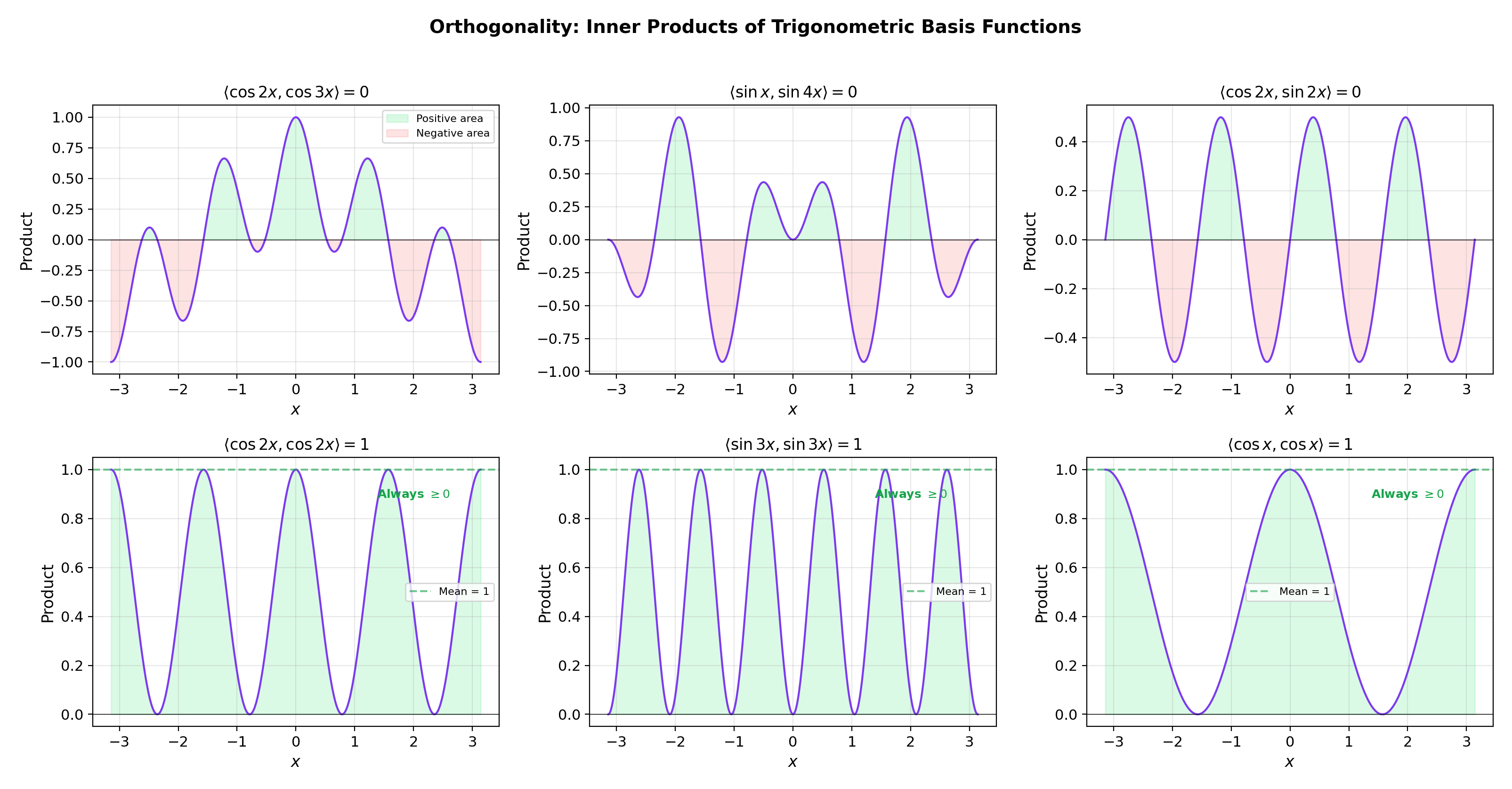
🔷 Theorem 1 (Orthogonality of the Trigonometric System)
The functions form an orthonormal system under :
for all , and , for , where is the Kronecker delta.
Proof.
By direct computation using product-to-sum formulas. For with :
since both and integrate to zero over a full period (as ). For :
The and cases follow similarly using the product-to-sum identities and .
📝 Example 5 (Orthogonality by direct computation)
Verify: . This is a specific instance of the general orthogonality: cosines and sines of different (or same) frequencies are always orthogonal.
💡 Remark 3 (Fourier coefficients as projections)
Orthogonality gives a coordinate formula. If , then taking the inner product with and using orthogonality:
Similarly . The Fourier coefficients are the orthogonal projections of onto each basis function — exactly as vector components are dot products with unit vectors in . The coefficient formulas in Definition 2 are not ad hoc; they are forced by orthogonality.
Try the explorer below — select two basis functions and watch how their pointwise product integrates to exactly 0 when the frequencies differ (the positive and negative areas cancel), and to exactly 1 when the frequencies match (the product is always non-negative).
4. Fourier Partial Sums & Pointwise Convergence
📐 Definition 5 (Fourier Partial Sum)
The th Fourier partial sum of is
This can be written as a convolution: where
is the Dirichlet kernel.
🔷 Theorem 3 (The Riemann-Lebesgue Lemma)
If is integrable on , then and as .
Proof.
For a step function , direct computation gives . Every integrable function can be approximated in the norm by step functions (from the definition of the Riemann integral). For general : given , choose a step function with . Then
Since , we get . Since is arbitrary, . The argument for is identical.
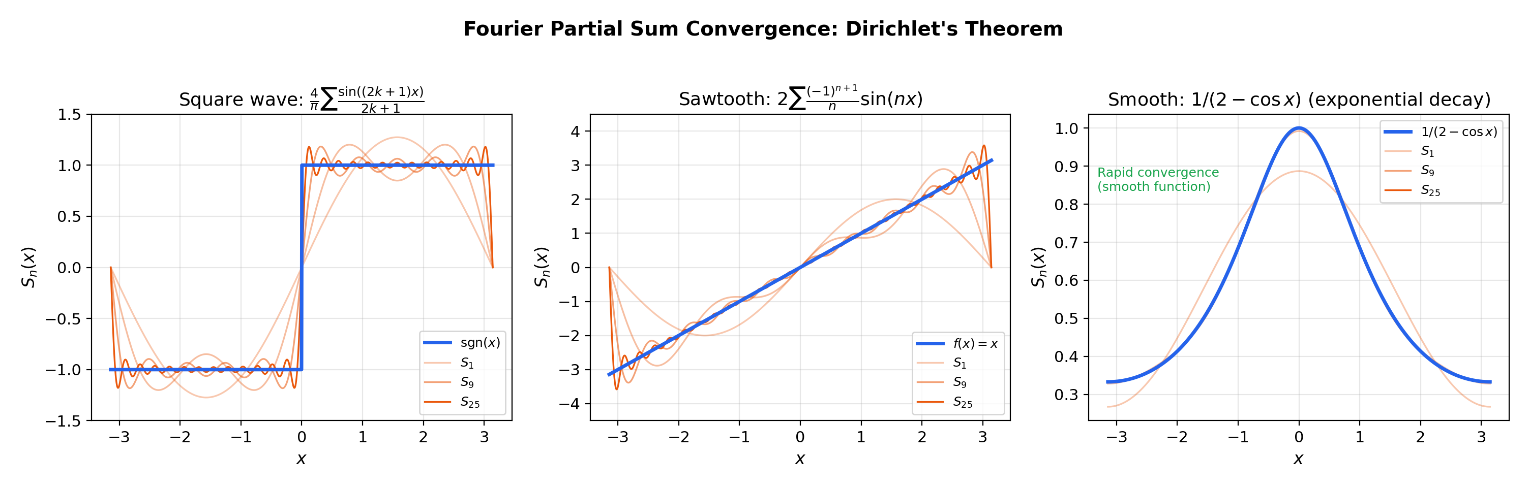
🔷 Theorem 4 (Dirichlet's Convergence Theorem)
If is piecewise smooth on (meaning and are piecewise continuous), then the Fourier series converges pointwise:
At points of continuity, this gives . At jump discontinuities, the partial sums converge to the average of the left and right limits.
📝 Example 4 (Square wave convergence)
At (discontinuity of ), Dirichlet’s theorem gives . At (point of continuity), .
💡 Remark 4 (The Dirichlet kernel and summation)
The Dirichlet kernel is the analog of the “evaluation functional” for Fourier series. As , concentrates near while oscillating rapidly elsewhere — a nascent delta function. The increasingly wild oscillations of are what cause convergence difficulties (including the Gibbs phenomenon in the next section). Compare with power series, where no such kernel appears because the monomial basis is not orthogonal under an integral inner product.
Drag the slider to watch the Fourier partial sums converge to each target function. Notice how convergence is fast for the smooth periodic function but painfully slow near the square wave’s discontinuities.
5. The Gibbs Phenomenon
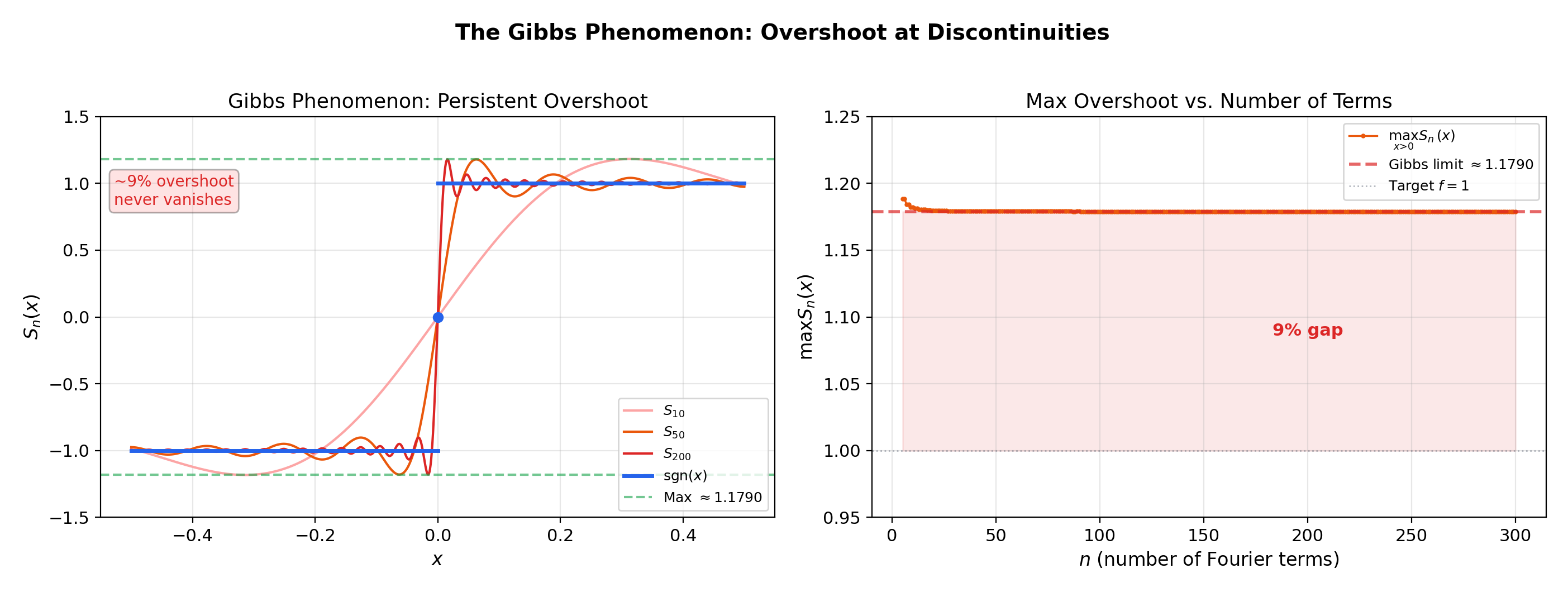
This is the most visually striking result in Fourier theory. Near a jump discontinuity, Fourier partial sums exhibit an overshoot that does not vanish as . The partial sums converge pointwise (Dirichlet’s theorem), but the maximum value near the jump overshoots by approximately 9%.
🔷 Proposition 2 (The Gibbs Phenomenon)
Let have a jump discontinuity at with jump height . Then the maximum of near overshoots the target value by approximately
The overshoot ratio is independent of — increasing compresses the overshoot into a narrower region near but does not reduce its height.
📝 Example 9 (Gibbs overshoot for the square wave)
The square wave has jump at . The maximum of near approaches approximately as , not . The location of the maximum moves toward as increases (at approximately ), but its height remains .
💡 Remark 5 (Gibbs vs. uniform convergence)
The Gibbs phenomenon means that is not uniform near a jump discontinuity, even though it is pointwise. This is fundamentally different from power series, where convergence inside the radius of convergence is uniform on compact subsets (Power Series & Taylor Series, Theorem 4). For Fourier series, uniform convergence requires global smoothness (see Section 7).
Increase in the explorer below and watch: the overshoot region gets narrower but the peak height stays at . The right panel confirms that the overshoot ratio converges to the Gibbs constant.
6. Coefficient Decay & Smoothness
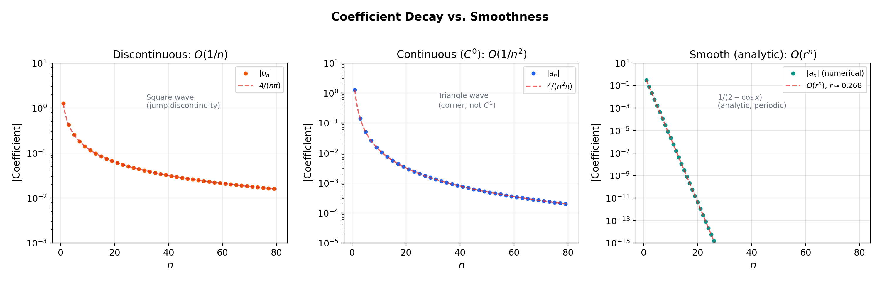
The central principle of Fourier analysis: smoothness of controls the decay rate of Fourier coefficients, and conversely.
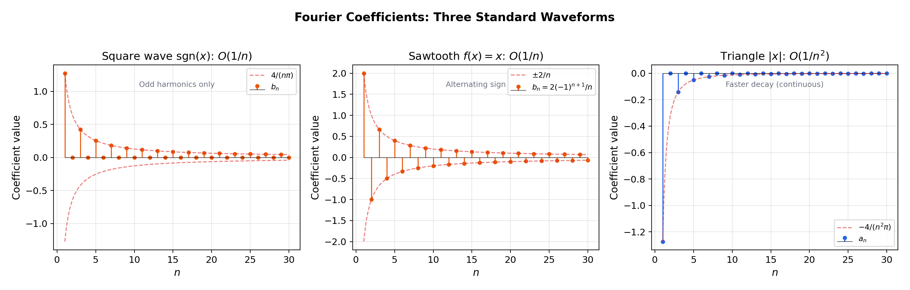
🔷 Proposition 1 (Coefficient Decay and Smoothness)
(a) If is (i.e., times continuously differentiable) and -periodic, then as . In particular:
- Discontinuous
- faster than any polynomial (superpolynomial decay)
(b) The mechanism: integration by parts times transfers powers of from the coefficient to the function. Specifically, if is and periodic, then the Fourier coefficients of satisfy , so where are the (bounded) coefficients of .
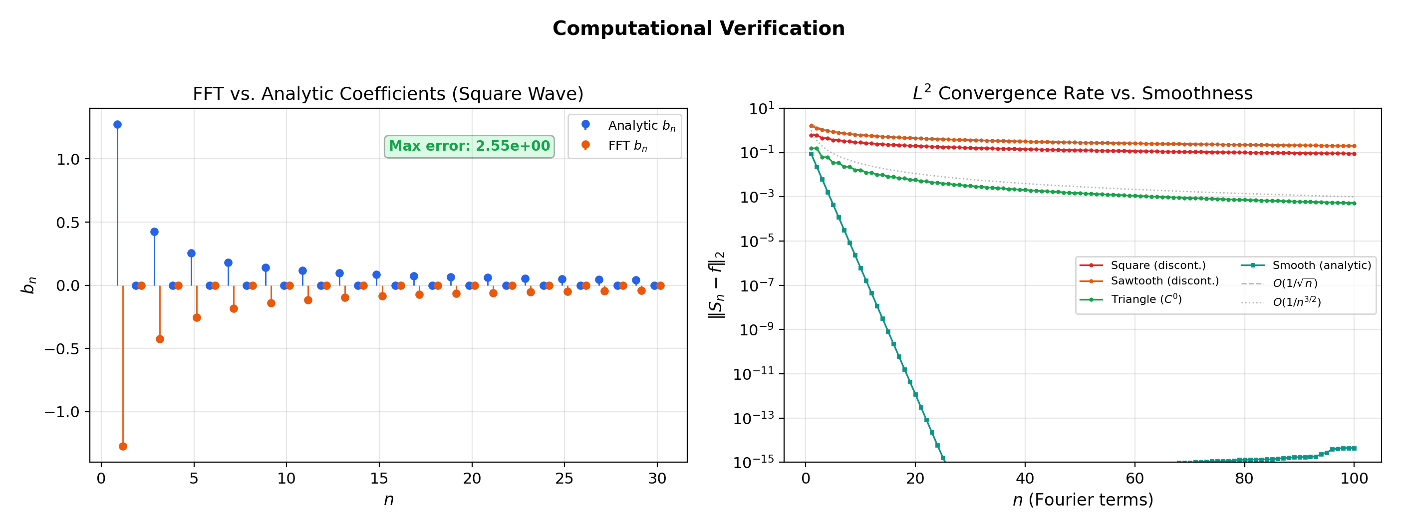
📝 Example 10 (Three decay regimes)
(a) The square wave has — discontinuous function, slowest possible decay.
(b) The triangle wave has — continuous but not differentiable (corner at ), one degree faster.
(c) The smooth periodic function has coefficients that decay exponentially: with . This is the Fourier counterpart of the smooth-vs-analytic distinction from Power Series & Taylor Series.
Compare the three decay regimes in the explorer. On a log scale, decay is a straight line with slope , has slope , and exponential decay drops off a cliff.
7. Uniform Convergence & Functions
🔷 Theorem 5 (Uniform Convergence under Smoothness)
If is (continuously differentiable) and -periodic, then the Fourier series of converges uniformly to .
More generally, if is continuous, -periodic, and the Fourier coefficients satisfy , then the Fourier series converges uniformly by the Weierstrass M-test from Uniform Convergence.
📝 Example 11 (Triangle wave — uniform but slow)
The triangle wave on has . Since (-series with from Series Convergence & Tests), the Fourier series converges uniformly to by the Weierstrass M-test. There is no Gibbs phenomenon because is continuous (though not differentiable). But the convergence rate is in the sup-norm — much slower than exponential convergence for smooth functions.
8. Bessel’s Inequality & Parseval’s Identity
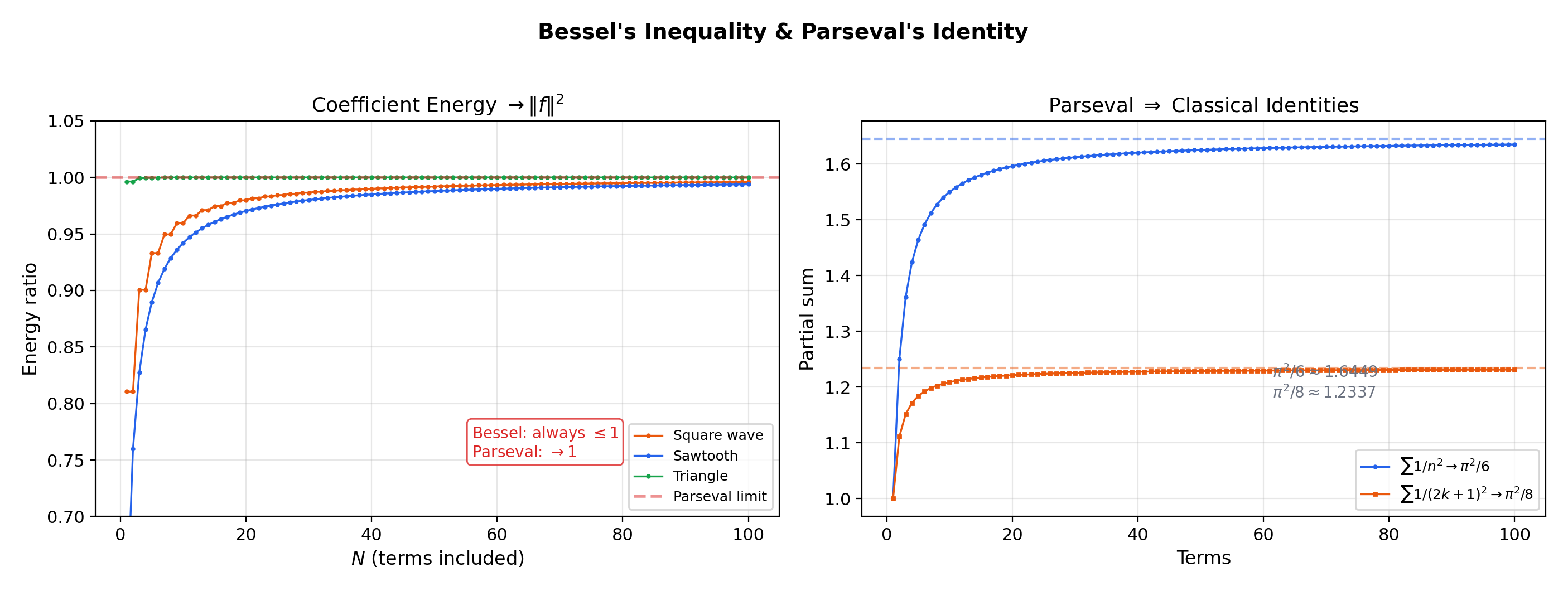
Energy conservation in the frequency domain. Bessel’s inequality says the energy in the Fourier coefficients cannot exceed the energy in . Parseval’s identity says equality holds — no energy is lost.
🔷 Theorem 2 (Bessel's Inequality)
For any integrable on ,
for every . Taking : .
Proof.
Expand :
By orthogonality, and . Substituting:
🔷 Theorem 6 (Parseval's Identity)
If is square-integrable on , then
Equality holds in Bessel’s inequality: no energy is lost in the Fourier decomposition.
📝 Example 6 (Bessel verification for the square wave)
The square wave has . With for odd , Parseval gives
which rearranges to — a non-trivial identity derived purely from Parseval.
📝 Example 7 (Parseval for the sawtooth — the Basel problem)
The sawtooth has . With , Parseval gives
which yields — the Basel problem, one of the most celebrated results in analysis, solved here by Fourier theory.
9. Term-by-Term Integration & Differentiation Caveats
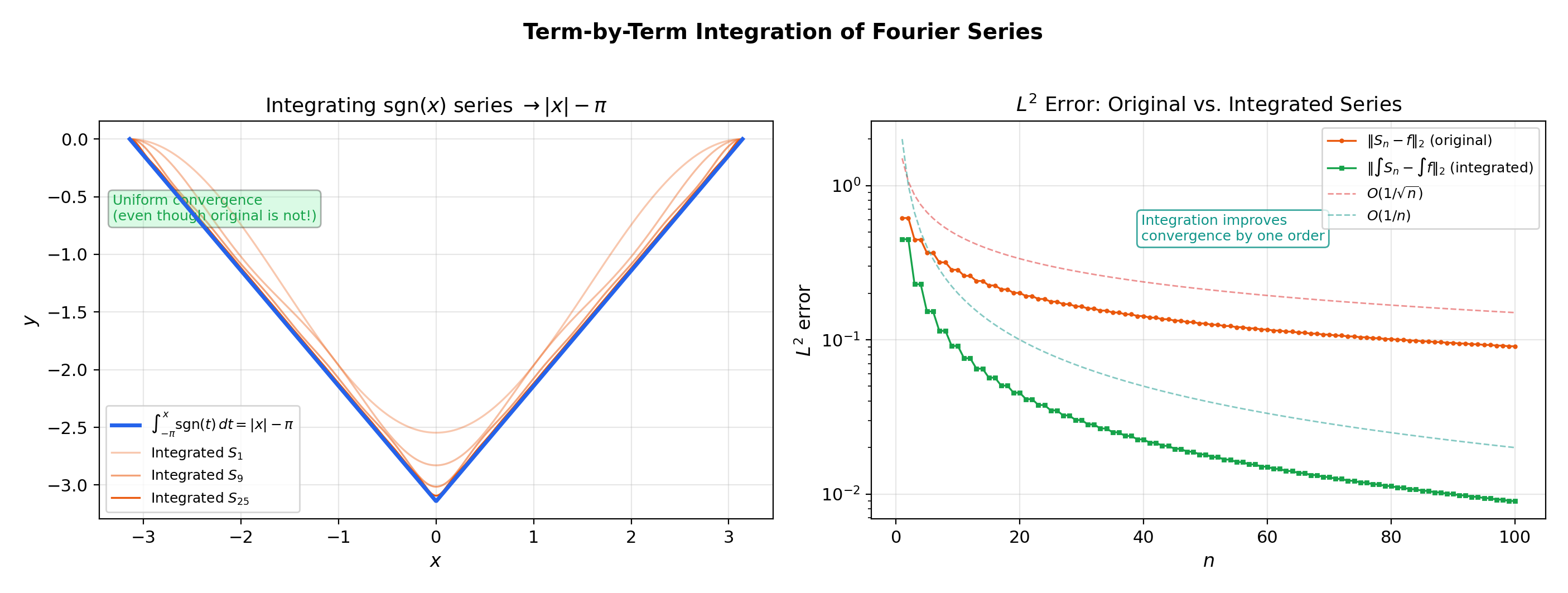
🔷 Theorem 7 (Term-by-Term Integration of Fourier Series)
If is integrable on with Fourier series , then for any :
The integrated series converges uniformly, even if the original Fourier series does not.
Proof.
The integrated series has coefficients and . By Bessel’s inequality from Theorem 2, . By Cauchy-Schwarz,
The Weierstrass M-test from Uniform Convergence then gives uniform convergence.
📝 Example 8 (Integrating the square wave)
Integrating from to gives
which converges uniformly — the integrated series of a non-uniformly convergent Fourier series is uniformly convergent. Integration improves convergence by one order.
💡 Remark 6 (Differentiation caveats)
Term-by-term differentiation of Fourier series is not generally valid. Differentiating the square wave’s Fourier series gives , which diverges everywhere. Differentiation multiplies the th coefficient by , making decay worse. For term-by-term differentiation to be valid, must be and periodic (so that also has a convergent Fourier series). Compare with power series, where differentiation preserves the radius of convergence — Fourier series are more delicate.
10. The Complex Exponential Form
💡 Remark 7 (Complex exponential form)
Using and , the Fourier series can be written
The complex form is more compact and connects directly to the Fourier transform (the non-periodic analog, extending this to all of ). In the complex form, Parseval’s identity becomes .
11. Connections to Statistics
Fourier analysis is the language of characteristic functions, kernel methods, and density estimation in the frequency domain. Every continuous distribution on is determined by its Fourier transform.
Characteristic functions and the CLT
Characteristic functions are Fourier transforms of densities. Lévy’s continuity theorem — convergence of characteristic functions implies convergence in distribution — is an application of Fourier inversion. The CLT is cleanest to prove via characteristic functions because Fourier analysis handles convolutions (sums of independent random variables) diagonally. See formalStatistics Central Limit Theorem.
KDE in the Fourier domain
The KDE’s characteristic function is the product of the data’s empirical characteristic function and the kernel’s Fourier transform. Plancherel’s identity converts the MISE spatial integral into a Fourier-side integral, clarifying bandwidth-selection asymptotics. See formalStatistics Kernel Density Estimation.
Continuous distributions
Every continuous distribution on is characterized by its Fourier transform. The Normal’s characteristic function is itself Gaussian — the analytical fact that makes the CLT proof so clean. See formalStatistics Continuous Distributions.
12. Connections to ML — Positional Encodings, Spectral Methods, Signal Processing
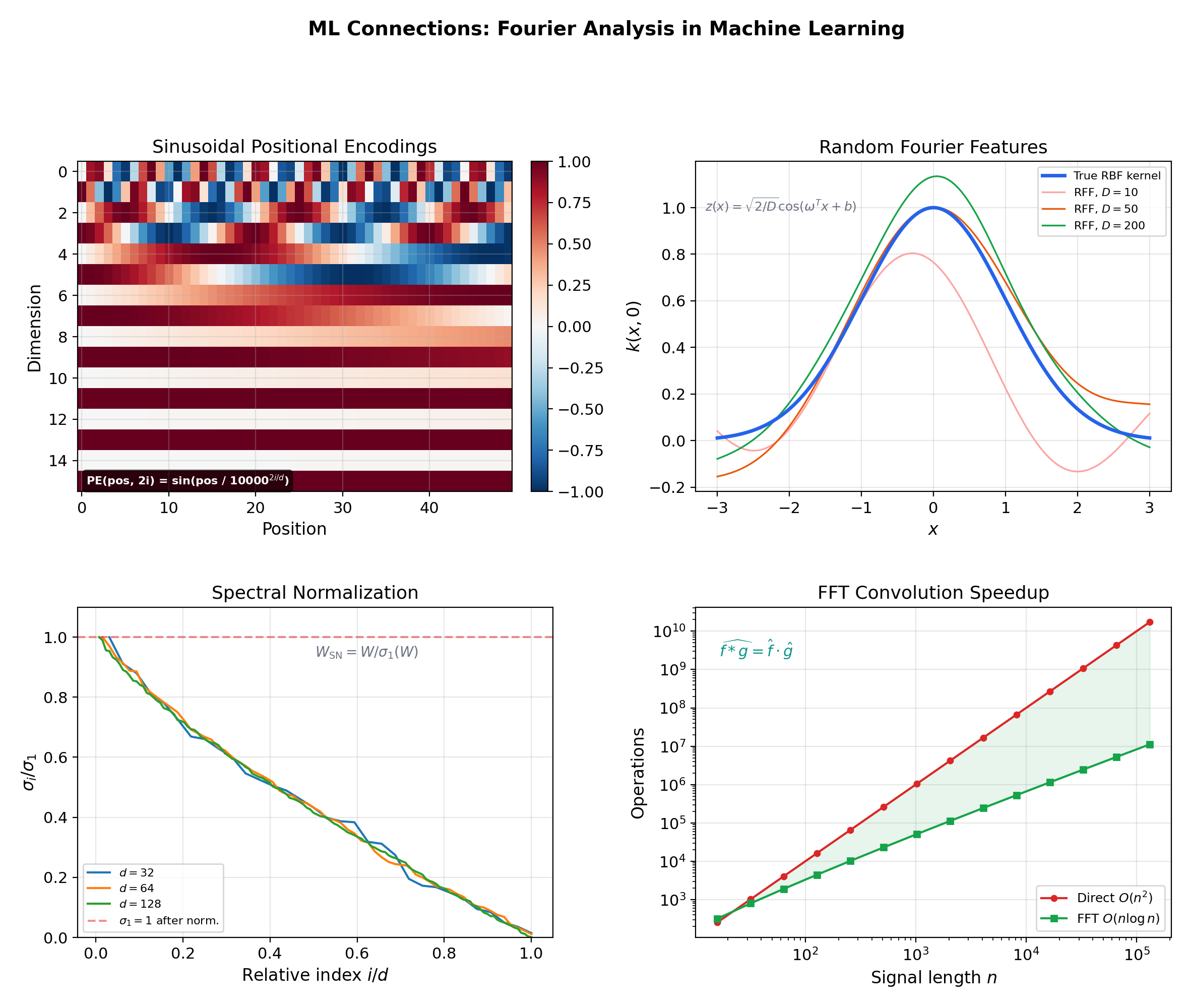
11.1. Sinusoidal positional encodings in transformers
The Transformer architecture encodes sequence position using
This is a Fourier basis at geometrically spaced frequencies. The orthogonality of the trigonometric system means the encoding at each frequency carries independent positional information. The choice of sinusoidal functions (rather than polynomial functions of position) enables the model to attend to relative positions via linear transformations — because and are linear combinations of .
→ formalML: PAC Learning — Fourier analysis on Boolean functions uses the same orthogonal decomposition structure.
11.2. Random Fourier Features
For shift-invariant kernels , Bochner’s theorem says for some probability measure . Random Fourier Features approximate the kernel using random trigonometric functions:
with and . Each random feature samples one Fourier coefficient of the kernel.
→ formalML: Gradient Descent — Random Fourier Features enable scalable kernel methods in optimization.
11.3. Spectral normalization
In GANs and deep networks, spectral normalization constrains the Lipschitz constant of each layer by dividing the weight matrix by its largest singular value. The singular values are the “spectral” (frequency-domain) quantities of the linear map — a generalization of Fourier analysis from functions to linear operators. Understanding Parseval’s identity (energy conservation under the Fourier transform) motivates why spectral normalization preserves representational power while constraining capacity.
11.4. Frequency-domain signal processing
Convolutional neural networks process signals in the spatial domain, but the convolution theorem says — convolution in the spatial domain is pointwise multiplication in the Fourier domain. Fast implementations of large-kernel convolutions use FFT to compute convolutions in rather than . The Fourier basis makes this possible because multiplication of Fourier coefficients is equivalent to function convolution.
13. Computational Notes
Fourier coefficient computation. For explicit functions, compute and analytically when possible; otherwise, use numerical quadrature. The trapezoidal rule is especially accurate for periodic functions — it converges exponentially for smooth periodic integrands, a fact that is itself a consequence of Fourier theory (the quadrature error depends on the Fourier coefficient decay of the integrand).
The FFT. The Fast Fourier Transform computes all discrete Fourier coefficients in operations, compared to for direct computation. This is used in practice for signal processing, image analysis, and spectral methods in PDEs.
Gibbs mitigation. Cesàro (Fejér) summation replaces with , which converges uniformly even at discontinuities — the Gibbs overshoot is smoothed out by averaging. The Lanczos sigma factor provides another smoothing approach. These techniques are used in spectral methods for PDEs where Gibbs oscillations corrupt numerical solutions.
Connections & Further Reading
Prerequisites — topics you need first
Power Series & Taylor Series
Power series use the monomial basis {xⁿ} for local approximation around a center c with radius of convergence R. Fourier series use the trigonometric basis {1, cos(nx), sin(nx)} for global periodic approximation on [−π, π]. The conceptual shift from local to global is the central theme of Topic 19.
The Riemann Integral & FTC
Fourier coefficients aₙ and bₙ are computed by Riemann integrals of f against cos(nx) and sin(nx). The inner product ⟨f,g⟩ = (1/π)∫f(x)g(x)dx is defined via the Riemann integral. Every Fourier coefficient computation is an integral computation.
Uniform Convergence
The Weierstrass M-test (Topic 4) establishes uniform convergence of Fourier series when coefficient decay is fast enough: if |aₙ|, |bₙ| ≤ Mₙ and Σ Mₙ < ∞, the Fourier series converges uniformly. The interchange theorems justify term-by-term integration.
Series Convergence & Tests
Bessel's inequality says Σ(aₙ² + bₙ²) converges — a series convergence statement about the coefficient sequence. The comparison test bounds the decay rates of coefficient sequences. The Riemann-Lebesgue lemma (aₙ → 0) is the Fourier analog of the divergence test's necessary condition.
Improper Integrals & Special Functions
The Riemann-Lebesgue lemma connects to improper integrals: ∫₋∞^∞ f(x)cos(ωx)dx → 0 as ω → ∞ for absolutely integrable f. Fourier coefficients on [−π,π] are the periodic version of this principle.
Where this leads — next in formalCalculus
Approximation Theory
Weierstrass approximation, Stone-Weierstrass, and best approximation in L² and C[a,b] — the theoretical home of the trigonometric approximation results sketched here.
Stability & Dynamical Systems
Fourier modes as eigenfunctions of the Laplacian — the spectral gap determines the convergence rate of diffusion on the circle, and the orthogonal decomposition makes stability analysis modal.
Lp Spaces
L² completeness (Riesz-Fischer) is what makes Fourier series rigorous orthogonal expansions in Hilbert space. The coefficients developed here are coordinates in an infinite-dimensional inner-product space.
Inner Product & Hilbert Spaces
The inner product defined here on L²[-π, π] is the prototype for abstract Hilbert space theory. The projection theorem generalizes the best-L²-approximation result from Section 5.
On to formalStatistics — where this calculus powers inference
Central Limit Theorem
Characteristic functions φ_X(t) = E[e^(itX)] are Fourier transforms of densities. Lévy's continuity theorem — convergence of characteristic functions implies convergence in distribution — is an application of Fourier inversion. The CLT is cleanest to prove via characteristic functions because Fourier analysis handles convolutions (sums of random variables) diagonally.
Kernel Density Estimation
The KDE's characteristic function is the product of the data's empirical characteristic function and the kernel's Fourier transform. Plancherel's identity ∫|f|² = ∫|F(f)|² converts the MISE spatial integral into a Fourier-side integral, clarifying bandwidth-selection asymptotics.
Continuous Distributions
Every continuous distribution on ℝ is characterized by its Fourier transform (characteristic function). The Normal's characteristic function e^(-σ²t²/2) is itself Gaussian — the analytical fact that makes the CLT proof so clean.
On to formalML — where this calculus powers ML
Gradient Descent
Random Fourier Features approximate shift-invariant kernels k(x−y) using random trigonometric functions z(x) = √(2/D)cos(ωᵀx + b). The kernel equals the Fourier transform of its spectral measure — random features are Monte Carlo estimates of Fourier coefficients.
Spectral Theorem
The Fourier decomposition f = Σ⟨f,eₙ⟩eₙ is the prototype for the spectral theorem for compact self-adjoint operators. The trigonometric system is the eigenbasis of the differentiation operator on the circle, and Fourier coefficients are eigencoordinates.
Information Geometry
Score functions in exponential families decompose into orthogonal components via the Fisher information inner product. The orthogonal projection structure of Fourier analysis carries over to the geometry of statistical manifolds.
PAC Learning
Fourier analysis on Boolean functions {−1,1}ⁿ uses Fourier coefficients f̂(S) = E[f(x)χ_S(x)] — the discrete analog of the continuous Fourier coefficients developed here. The KKL inequality and noise sensitivity bounds are proved via Fourier-analytic methods.
References
- book Rudin (1976). Principles of Mathematical Analysis Chapter 8 — Fourier series, orthogonality, Parseval's theorem, and the Dirichlet kernel
- book Stein & Shakarchi (2003). Fourier Analysis: An Introduction Chapters 2-3 — the definitive modern treatment of Fourier series convergence, Gibbs phenomenon, and applications
- book Abbott (2015). Understanding Analysis Chapter 8 — Fourier series with emphasis on pointwise vs. uniform convergence and the role of the inner product
- book Folland (1999). Real Analysis: Modern Techniques and Their Applications Section 8.2 — Fourier series in the L² framework, Parseval's identity, and completeness of the trigonometric system
- book Spivak (2008). Calculus Chapter 15 — trigonometric functions and their orthogonality, with careful treatment of Fourier coefficient computation
- paper Vaswani, Shazeer, Parmar, Uszkoreit, Jones, Gomez, Kaiser & Polosukhin (2017). “Attention Is All You Need” Sinusoidal positional encodings PE(pos, 2i) = sin(pos/10000^(2i/d)) use the Fourier basis to encode sequence position — a direct application of the orthogonal trigonometric system to representation learning.
- paper Rahimi & Recht (2007). “Random Features for Large-Scale Kernel Machines” Random Fourier Features approximate shift-invariant kernels via Monte Carlo sampling of Fourier coefficients: z(x) = √(2/D)cos(ωᵀx + b) with ω drawn from the spectral distribution.