Stability & Dynamical Systems
When eigenvalues predict the future — linearization, Lyapunov functions, bifurcations, and the qualitative theory that tells you whether trajectories converge, diverge, or orbit forever.
Abstract. Stability analysis is the qualitative theory of differential equations — the art of predicting long-term behavior without solving the ODE explicitly. The linearization stability theorem connects the eigenvalues of the Jacobian at an equilibrium to the local phase portrait, reducing nonlinear analysis to the linear classification from Topic 22. Lyapunov's direct method provides a complementary energy-based approach: if a scalar function V decreases along trajectories, the system is stable. Bifurcation theory asks what happens when parameters change — equilibria can appear, disappear, or exchange stability at critical thresholds. These tools are the mathematical backbone of gradient descent convergence analysis, GAN training dynamics, and neural ODE stability.
1. What Happens Next?
You train a neural network and the loss plateaus. Is it stuck at a local minimum — a stable equilibrium where gradient descent has settled in? Is it perched on a saddle point, about to escape along some direction you haven’t explored yet? Or is it approaching a slow-converging valley where the landscape is nearly flat?
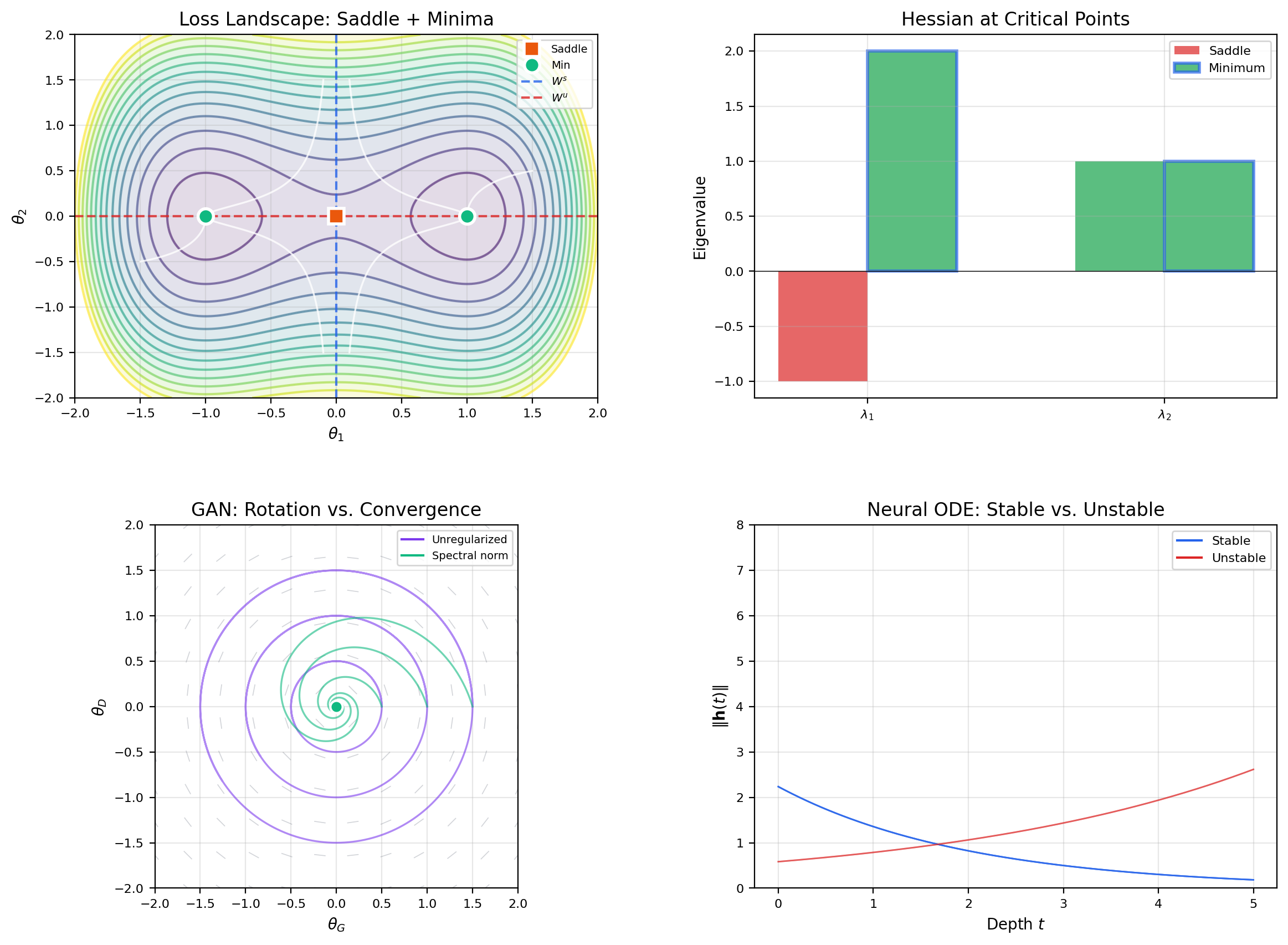
The answer depends on the eigenvalues of the Hessian at the critical point. All eigenvalues positive means stable minimum. Any eigenvalue negative means saddle — the corresponding eigenvector points along the escape route. Near-zero eigenvalues mean near-degeneracy — convergence along those directions is glacially slow.
This is exactly the linearization stability theorem applied to the gradient flow ODE . The Jacobian of the right-hand side at a critical point is , and its eigenvalues — the negatives of the Hessian eigenvalues — determine local stability.
This topic develops the complete qualitative theory of differential equations. We build three tools:
- Linearization — reduce a nonlinear system to a linear one near an equilibrium by computing the Jacobian. The eigenvalue classification from Topic 22 tells us the local behavior.
- Lyapunov functions — find a scalar “energy” function that decreases along trajectories. If such a function exists, the system is stable — no need to solve the ODE.
- Bifurcation theory — study how qualitative behavior changes as parameters vary. Equilibria can appear, disappear, or exchange stability at critical thresholds.
Together, these tools explain why gradient descent converges, why GANs oscillate, and why learning rate schedules work.
2. Equilibria & Nullclines
We work with autonomous 2D systems: , , written compactly as .
📐 Definition 1 (Equilibrium Point (Stationary Point, Fixed Point))
A point is an equilibrium of if . If , then for all — the system stays put.
Finding equilibria means solving and simultaneously. For nonlinear systems, this can be difficult. Nullclines make the search geometric.
📐 Definition 2 (Nullcline)
The -nullcline (or -nullcline) is the curve . On this curve, — trajectories move purely vertically. Similarly, the -nullcline is , where trajectories move purely horizontally. Equilibria occur where the nullclines intersect.
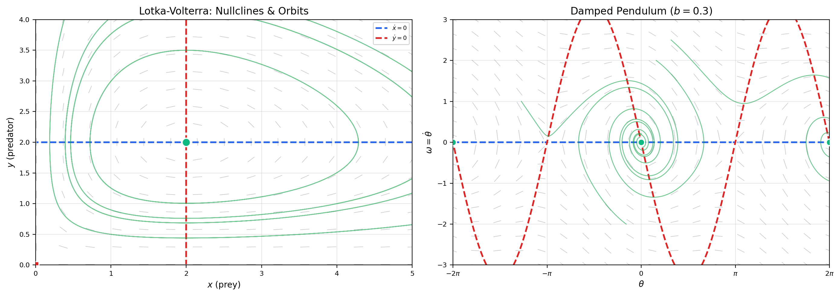
📝 Example 1 (Lotka-Volterra Equilibria and Nullclines)
The predator-prey system is: where is prey population, is predator population, and .
-nullcline: , so or .
-nullcline: , so or .
Equilibria are the intersections:
- — both species extinct (trivial equilibrium)
- — coexistence equilibrium
The nullclines divide the positive quadrant into four regions, and in each region we can determine the direction of the flow by checking the sign of and . This gives a coarse picture of the dynamics without solving anything.
📝 Example 2 (Damped Pendulum Equilibria)
The damped pendulum becomes a first-order system:
-nullcline: (the -axis).
-nullcline: (an S-shaped curve through the origin).
Equilibria: and , giving for all integers . The pendulum has infinitely many equilibria — the downward rest positions and the upward balance points .
💡 Remark 1 (Nullclines Reduce a 2D Search to Curve Intersections)
Without nullclines, finding equilibria requires solving two nonlinear equations simultaneously — a 2D root-finding problem. Nullclines reduce this to a 1D problem: trace each nullcline as a curve, then find where they cross. The flow directions between nullclines then give a rough sketch of the phase portrait for free.
3. The Linearization Stability Theorem
We now develop the fundamental tool for classifying equilibria of nonlinear systems. The idea: near an equilibrium, a nonlinear system looks like a linear system, and we already know how to classify linear systems from Topic 22.
📐 Definition 3 (Stability, Asymptotic Stability, and Instability (Lyapunov))
Let be an equilibrium of .
-
is stable (in the sense of Lyapunov) if for every there exists such that implies for all . Trajectories starting close stay close.
-
is asymptotically stable if it is stable and additionally as for all sufficiently close to . Trajectories starting close converge to the equilibrium.
-
is unstable if it is not stable — some trajectories starting arbitrarily close eventually leave a neighborhood of .
📐 Definition 4 (Hyperbolic Equilibrium)
An equilibrium is hyperbolic if every eigenvalue of the Jacobian has nonzero real part: for all . In the language of Topic 22, the linearized system has no center component — it is a node, saddle, or spiral, never a center.
Here is the main theorem. It says that at a hyperbolic equilibrium, linearization tells the whole story.
🔷 Theorem 1 (Linearization Stability Theorem (Hartman-Grobman, Stability Version))
Let be an equilibrium of with continuously differentiable, and let be the Jacobian at .
- If all eigenvalues of satisfy , then is asymptotically stable.
- If any eigenvalue of satisfies , then is unstable.
- If all eigenvalues have (the equilibrium is hyperbolic), the phase portrait near is qualitatively equivalent to that of the linear system .
Proof.
We prove statement (1); statement (2) follows by a time-reversal argument.
Set . Taylor expansion gives: where the remainder satisfies for sufficiently small (since is ).
Step 1: The linear part decays exponentially. Since all eigenvalues of have , there exist constants and such that for all . (This uses the Jordan normal form and the fact that can be taken as any number smaller than .)
Step 2: Variation of constants formula. The solution of satisfies the integral equation:
Step 3: Gronwall estimate. Let . Then:
For sufficiently small (say with ), a continuation argument shows that for all .
Specifically: suppose on . Then on this interval:
By Gronwall’s inequality, if , the integral term does not overcome the exponential decay of the first term. The bound holds on , and since the bound does not saturate, it extends beyond — by continuity, the bound holds for all .
Conclusion: exponentially, so is asymptotically stable.
📝 Example 3 (Classify Lotka-Volterra Equilibria via Linearization)
From Example 1, the Lotka-Volterra system , has equilibria at and .
The Jacobian is:
At : . Eigenvalues: , . This is a saddle point — unstable. The prey axis is the unstable manifold (prey grow exponentially without predators); the predator axis is the stable manifold (predators die without prey).
At : . The eigenvalues are — pure imaginary. This is a non-hyperbolic center in the linearization. Linearization is inconclusive! (In fact, the nonlinear system has a conserved quantity, so the orbits are genuinely closed — but the linearization cannot tell us this.)
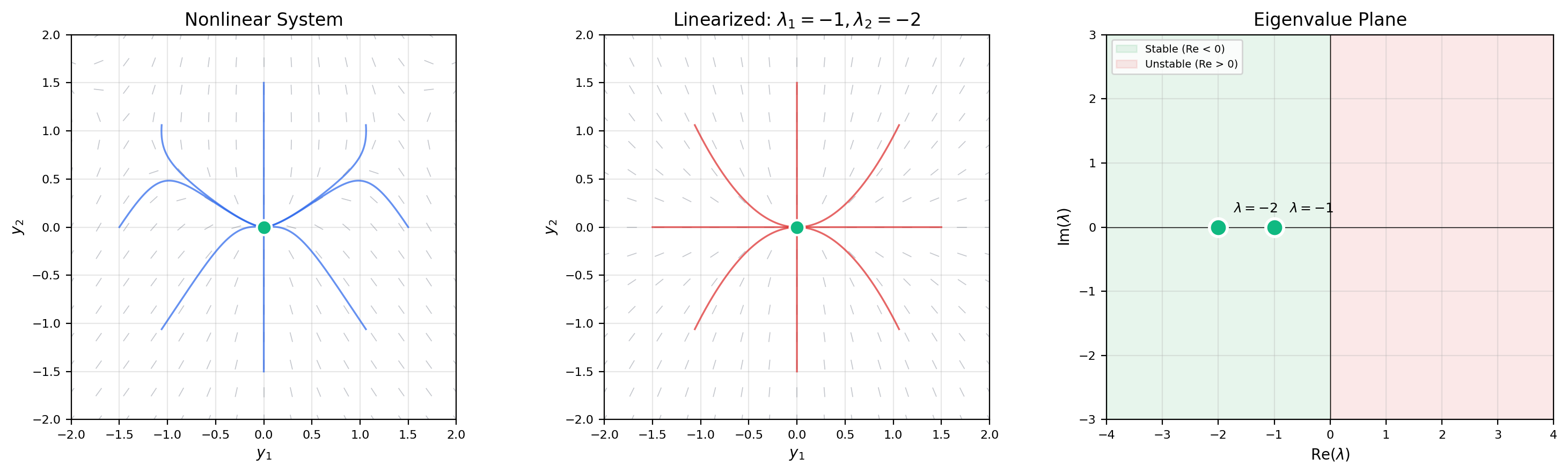
📝 Example 4 (Non-Hyperbolic Case — Center vs. Spiral)
Consider the family:
The Jacobian at the origin is with eigenvalues .
- For : → stable spiral (linearization is conclusive).
- For : → linearization gives a center, but the nonlinear cubic terms create a stable spiral (trajectories decay).
- For : → unstable spiral (linearization is conclusive), and a stable limit cycle of radius appears.
The non-hyperbolic case shows that linearization alone cannot distinguish a true center from a spiral when eigenvalues are pure imaginary. We need Lyapunov functions (Section 4) or the Hopf bifurcation theorem (Section 8).
💡 Remark 2 (Hyperbolicity as a Genericity Condition)
Non-hyperbolic equilibria are “exceptional” — they require eigenvalues to land exactly on the imaginary axis, which is a codimension-one condition in parameter space. Generically (for “almost all” parameter values), all equilibria are hyperbolic. Non-hyperbolic equilibria typically occur at bifurcation points — the boundaries between qualitatively different behaviors (Section 8).
4. Lyapunov’s Direct Method
Linearization classifies equilibria using the Jacobian’s eigenvalues — a local, algebraic test. Lyapunov’s direct method takes a completely different approach: find a scalar “energy” function that decreases along trajectories. If such a function exists, the system is stable, and we never need to solve the ODE or compute eigenvalues.
The key is the orbital derivative: if is a smooth scalar function and is a solution of , then by the chain rule:
This is computable directly from and — we don’t need the solution .
📐 Definition 5 (Lyapunov Function)
A continuously differentiable function defined on a neighborhood of an equilibrium is a Lyapunov function if:
- and for in (positive-definite)
- in (negative-semidefinite orbital derivative)
If additionally for (negative-definite), then is a strict Lyapunov function.
🔷 Theorem 2 (Lyapunov Stability Theorem)
Let be an equilibrium of .
- If there exists a Lyapunov function with , then is stable.
- If there exists a strict Lyapunov function with for , then is asymptotically stable.
Proof.
We prove statement (1). Statement (2) follows by a similar argument with the additional conclusion that forces .
Goal: For every , find such that implies for all .
Step 1: Sublevel set confinement. Fix and consider the compact set (the sphere of radius ). Since is continuous and positive on , it attains a minimum:
Step 2: Choose . Since and is continuous, there exists (with ) such that implies .
Step 3: Trajectories stay inside. Suppose , so . Since along trajectories:
If the trajectory were to reach , we would have — a contradiction. Therefore for all .
🔷 Theorem 3 (LaSalle's Invariance Principle)
Suppose is a Lyapunov function with on a compact positively invariant set . Let , and let be the largest invariant set contained in . Then every trajectory starting in converges to as .
In particular, if the only invariant subset of is , then is asymptotically stable — even though may vanish on a larger set.
📝 Example 5 (Damped Pendulum Energy as a Lyapunov Function)
For the damped pendulum , with , the total energy is:
This is positive-definite near : and for when .
The orbital derivative is:
So is a Lyapunov function and the origin is stable. But on the set — not just at the origin. Is it asymptotically stable?
LaSalle’s principle to the rescue: The largest invariant set in is just , because if for all then , forcing , hence (near the origin). By LaSalle’s principle, is asymptotically stable.
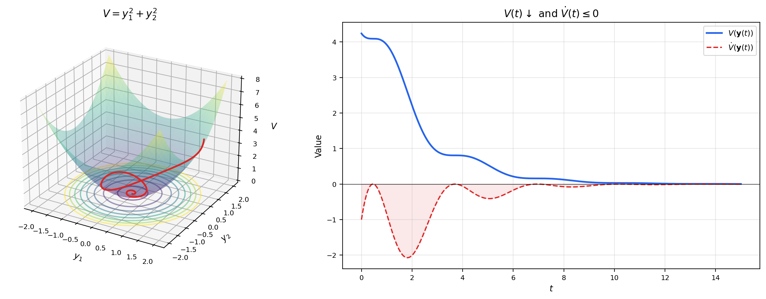
📝 Example 6 (Computing the Orbital Derivative for a Quadratic Lyapunov Function)
Consider the system , with candidate .
The gradient is , and the orbital derivative is:
Since for , is a strict Lyapunov function and the origin is asymptotically stable. The decay rate is , so — exponential convergence.
💡 Remark 3 (Finding Lyapunov Functions is an Art)
There is no systematic method for constructing Lyapunov functions for general nonlinear systems. Common strategies include:
- Physical energy (kinetic + potential) for mechanical systems
- Quadratic forms for systems near a linear regime (see Section 5)
- Sum-of-squares (SOS) programming — a computational approach using semidefinite optimization
- Trial and error guided by the structure of
The art is in finding a whose level curves “match” the dynamics well enough that comes out negative-definite. This is one place where understanding the physics or geometry of a system genuinely helps.
5. The Lyapunov Equation & Quadratic Lyapunov Functions
For linear systems , Lyapunov functions can be constructed systematically. The key is the quadratic form , where is a symmetric positive-definite matrix.
The orbital derivative is:
If we can choose so that for some positive-definite , then for — a strict Lyapunov function.
📐 Definition 6 (Hurwitz Matrix)
A matrix is Hurwitz (or stable) if every eigenvalue has strictly negative real part: for all . Equivalently, is Hurwitz if and only if as .
🔷 Theorem 4 (The Lyapunov Equation)
Let be a real matrix and a symmetric positive-definite matrix. The matrix equation has a unique symmetric positive-definite solution if and only if is Hurwitz.
When is Hurwitz, is a strict Lyapunov function for , confirming asymptotic stability.
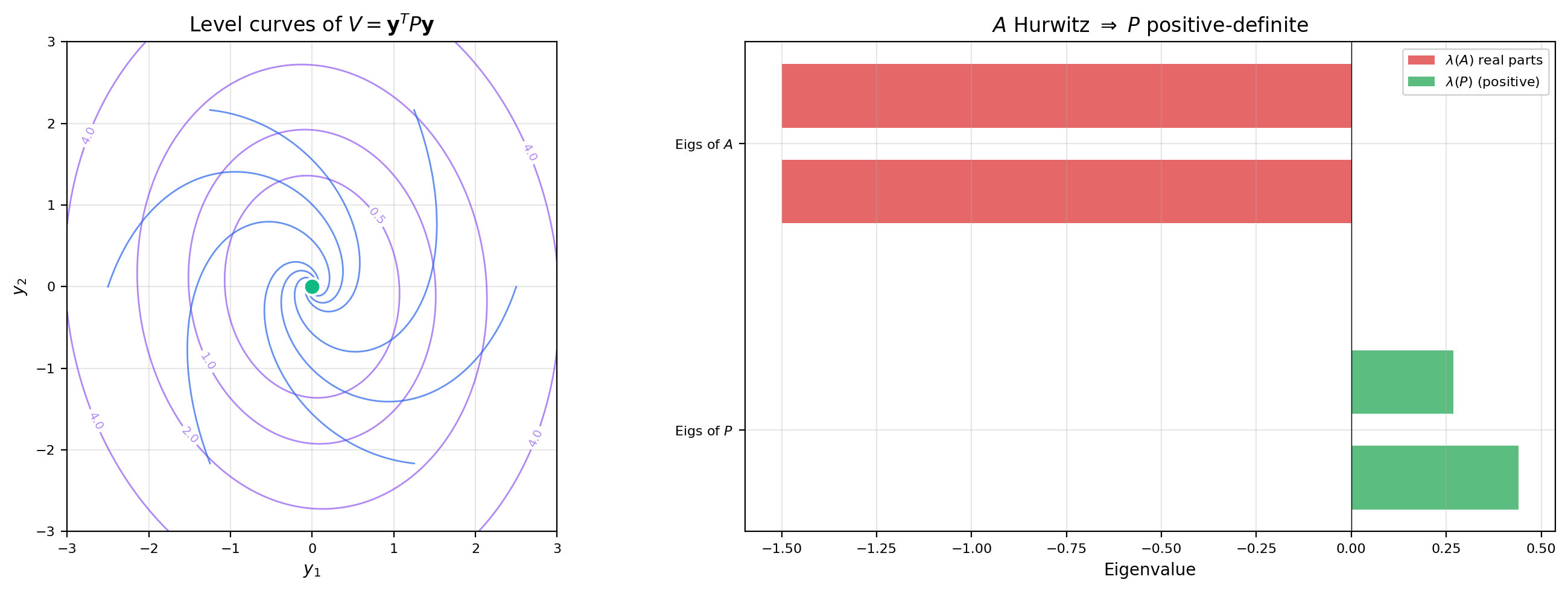
📝 Example 7 (Solving the Lyapunov Equation for a 2×2 Hurwitz Matrix)
Let . The eigenvalues are — both have negative real part, so is Hurwitz.
Choose (the simplest positive-definite choice). The Lyapunov equation is a linear system in the entries of :
Solving: . The eigenvalues of are approximately and , both positive — confirming .
The Lyapunov function has elliptical level curves, and .
📝 Example 8 (Quadratic Lyapunov Function for Training Dynamics)
Gradient descent on the quadratic loss yields the linear system . If is positive-definite (a local minimum), then is Hurwitz.
The loss function itself is a Lyapunov function: with . This proves gradient descent converges — the loss decreases monotonically along the gradient flow.
More precisely, solves (the Lyapunov equation with ). The condition number controls the eccentricity of the level ellipses — ill-conditioned Hessians produce elongated ellipses where gradient descent zig-zags.
💡 Remark 4 (The Lyapunov Equation as a Linear System)
The Lyapunov equation can be rewritten using the Kronecker product:
This is a linear system of size , solvable by standard methods. In Python: scipy.linalg.solve_continuous_lyapunov(A.T, -Q). The condition for unique solvability is that and share no eigenvalues — which holds precisely when is Hurwitz (since then all eigenvalues of have negative real parts, while eigenvalues of have positive real parts).
6. Invariant Manifolds
At a saddle-type equilibrium, some directions attract trajectories while others repel them. The invariant manifolds organize these directions into global geometric structures.
📐 Definition 7 (Stable and Unstable Manifolds)
Let be a hyperbolic equilibrium of .
-
The stable manifold is — the set of initial conditions that converge to in forward time.
-
The unstable manifold is — the set of initial conditions that converge to in backward time (equivalently, trajectories that depart from in forward time).
🔷 Theorem 5 (Stable Manifold Theorem)
Let be a hyperbolic equilibrium of with . Let have eigenvalues with negative real part and eigenvalues with positive real part. Then:
- is a smooth manifold of dimension , tangent to the stable eigenspace of at .
- is a smooth manifold of dimension , tangent to the unstable eigenspace of at .
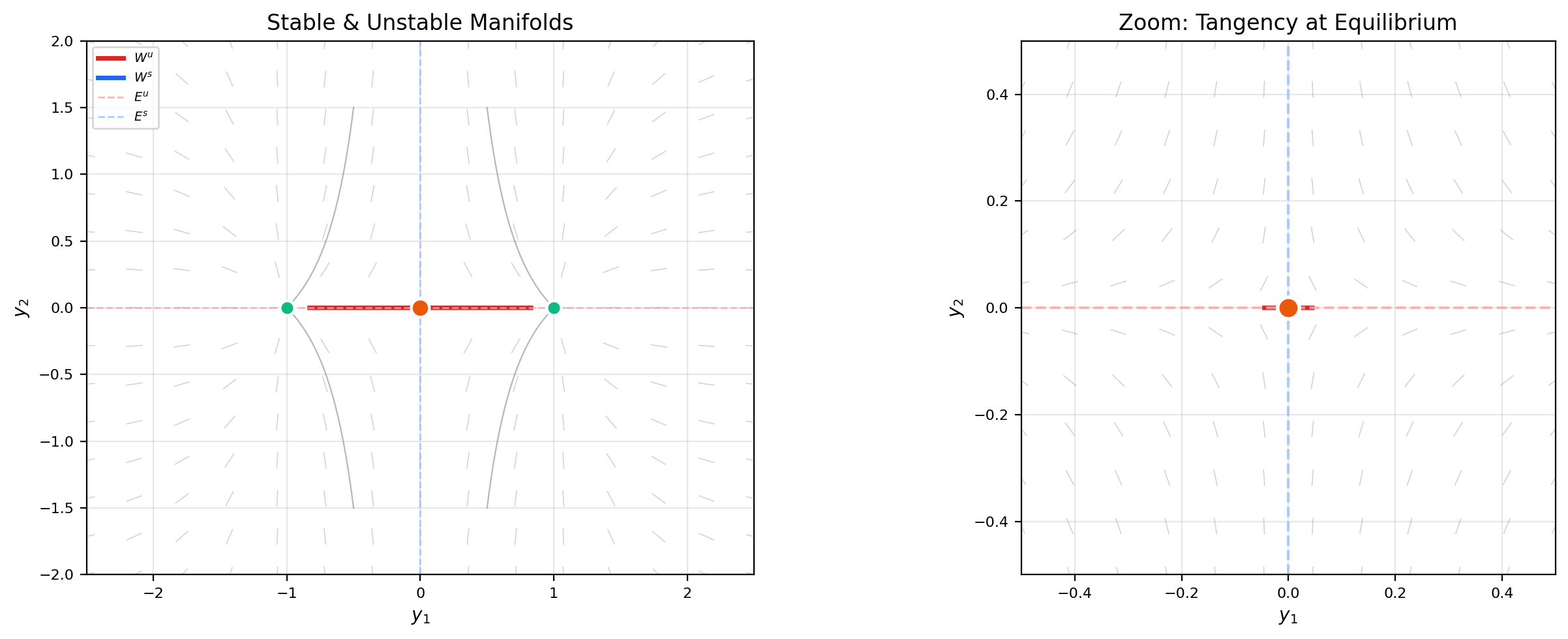
📝 Example 9 (Stable and Unstable Manifolds of a Lotka-Volterra Saddle)
At the origin of the Lotka-Volterra system, the Jacobian has eigenvalues (unstable, prey direction) and (stable, predator direction).
The stable manifold is the positive -axis: . Predators with no prey die exponentially — trajectories along this axis converge to the origin.
The unstable manifold is the positive -axis: . Prey with no predators grow exponentially — trajectories along this axis depart from the origin.
Both manifolds are straight lines — they coincide with the eigenspaces of the Jacobian. For nonlinear systems in general, the manifolds are curves (not lines) that are tangent to the eigenspaces at the equilibrium but curve away from them further out.
💡 Remark 5 (Center Manifolds and Dimensional Reduction)
When the Jacobian has eigenvalues on the imaginary axis (), the center manifold captures the “slow” dynamics that linearization cannot resolve. The center manifold theorem states that exists, is tangent to the center eigenspace at the equilibrium, and is locally invariant. The dynamics restricted to determine the stability of the full system — this is the principle of dimensional reduction: reduce the analysis to the center manifold, where the essential nonlinearity lives.
7. Limit Cycles & the Poincaré-Bendixson Theorem
Linear systems can have periodic orbits — the centers of Topic 22, where trajectories form closed ellipses. But these orbits are not isolated: every nearby initial condition also produces a periodic orbit. Limit cycles are a fundamentally nonlinear phenomenon: isolated periodic orbits that attract (or repel) neighboring trajectories.
📐 Definition 8 (Limit Cycle)
A limit cycle is an isolated closed orbit of .
- Stable limit cycle: Nearby trajectories spiral toward from both inside and outside. is an attractor.
- Unstable limit cycle: Nearby trajectories spiral away from .
- Semi-stable limit cycle: Trajectories approach from one side and recede on the other.
🔷 Theorem 6 (Poincaré-Bendixson Theorem)
Let be a planar system. If a trajectory remains in a bounded region for all , and contains no equilibria, then the -limit set of the trajectory is a periodic orbit.
More generally: if the -limit set is nonempty, compact, and contains no equilibria, it is a periodic orbit.
Proof.
The full proof is long and uses delicate topological arguments about planar flows. We outline the key ideas.
Step 1: -limit set structure. The -limit set is nonempty (by boundedness), compact, connected, and invariant under the flow.
Step 2: No equilibria in . By hypothesis, contains no equilibria. Therefore every point of lies on a regular orbit arc.
Step 3: Flow box and transversal. At any point , the flow is locally a parallel flow (by the Flow Box Theorem). Take a small transversal segment through . The trajectory must cross repeatedly (since is an -limit point).
Step 4: Monotonicity on . The Jordan Curve Theorem constrains how the trajectory can cross : successive crossings must be monotone (each crossing is “closer” to than the last). This is where 2D topology is essential — and why the theorem fails in 3D.
Step 5: Convergence. The monotone sequence of crossings converges to a fixed point on , which lies on a periodic orbit in . Since is connected and contains no equilibria, the entire -limit set equals this periodic orbit.
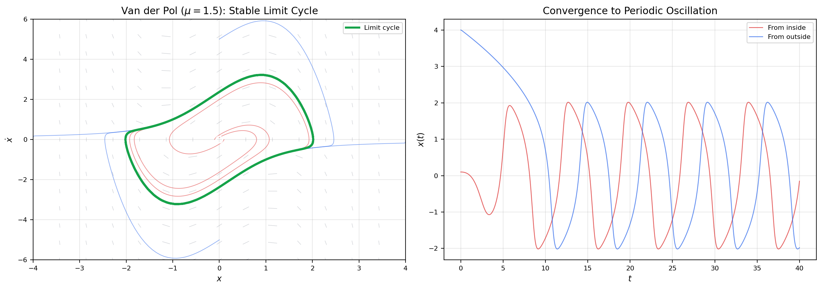
📝 Example 10 (Van der Pol Limit Cycle — Trapping Region)
The Van der Pol oscillator (with ) becomes:
Linearization at origin: The Jacobian has eigenvalues . For , — the origin is an unstable spiral (or unstable node for ).
Trapping region: Construct a bounded, positively invariant annular region surrounding the origin that contains no equilibria (the only equilibrium is the origin, which is excluded). By the Poincaré-Bendixson theorem, must contain a periodic orbit — the Van der Pol limit cycle.
For small, the limit cycle is nearly circular with radius . As increases, it develops sharp corners — the characteristic relaxation oscillation shape.
💡 Remark 6 (Poincaré-Bendixson is Special to 2D)
The Poincaré-Bendixson theorem critically uses 2D topology — the Jordan Curve Theorem, which has no analog in higher dimensions. In 3D, bounded trajectories that avoid equilibria need not converge to periodic orbits. Instead, they can exhibit chaotic behavior: the Lorenz attractor (, , ) is bounded, has no periodic orbits, and is a strange attractor with sensitive dependence on initial conditions. Chaos is impossible in 2D autonomous systems — a fundamental constraint of planar topology.
8. Bifurcation Theory
So far we’ve asked: given a system, what is the long-term behavior? Bifurcation theory asks a deeper question: how does the behavior change as a parameter varies? A bifurcation occurs when the qualitative structure of the phase portrait changes — equilibria appear or disappear, or exchange stability.
📐 Definition 9 (Bifurcation and Bifurcation Point)
A bifurcation of occurs at a parameter value if the phase portrait for near is not qualitatively equivalent to the phase portrait at . The value is a bifurcation point.
Typical signatures: the number of equilibria changes, or an equilibrium changes stability (eigenvalues cross the imaginary axis).
📐 Definition 10 (Saddle-Node Bifurcation (Normal Form))
The saddle-node bifurcation has normal form (in 1D) or , (in 2D).
- For : two equilibria at — one stable node, one saddle.
- At : the equilibria merge into a single half-stable equilibrium at .
- For : no equilibria — all trajectories escape.
Two equilibria collide, annihilate, and disappear as decreases through zero.
📐 Definition 11 (Hopf Bifurcation (Supercritical and Subcritical))
A Hopf bifurcation occurs when a pair of complex conjugate eigenvalues of the Jacobian crosses the imaginary axis: with (transversality).
- Supercritical Hopf: For , a stable equilibrium. At , the equilibrium loses stability and a stable limit cycle is born. The limit cycle grows as .
- Subcritical Hopf: For , a stable equilibrium coexists with an unstable limit cycle. At , the limit cycle shrinks to zero and the equilibrium becomes unstable — often accompanied by a sudden jump to a distant attractor.
🔷 Theorem 7 (Hopf Bifurcation Theorem)
Let have an equilibrium with Jacobian eigenvalues . Suppose:
- and (eigenvalues on imaginary axis)
- (transversal crossing)
Then a branch of periodic orbits bifurcates from at . The period is approximately and the amplitude scales as .
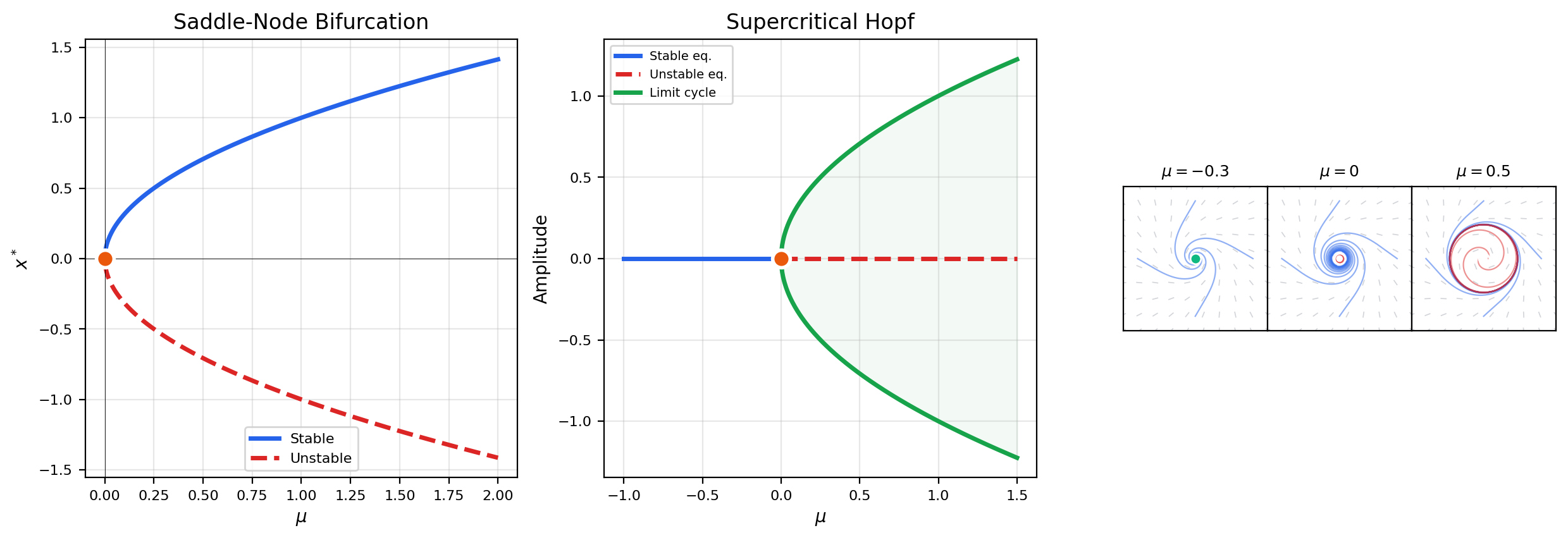
📝 Example 11 (Saddle-Node Bifurcation — Complete Analysis)
Consider on .
Equilibria: (exist only for ).
Stability: , so (stable) and (unstable).
Bifurcation diagram: Plot vs. . The curve (upper branch, stable, solid line) and (lower branch, unstable, dashed line) meet at the origin — the bifurcation point. The branches form a parabola opening to the right.
At the bifurcation (): The linearization is — a non-hyperbolic equilibrium. The system slows down critically: trajectories approach algebraically () rather than exponentially.
📝 Example 12 (Supercritical Hopf — Birth of a Limit Cycle)
The Hopf normal form:
In polar coordinates : , .
Equilibria of the radial equation: (always) and (for ).
- : Only exists. Since for , the origin is asymptotically stable (stable spiral).
- : The origin is non-hyperbolic. The cubic term stabilizes it weakly.
- : is unstable, is a stable limit cycle. Every trajectory (except the origin itself) spirals toward the circle of radius .
The limit cycle amplitude grows as — a square-root scaling that is universal for supercritical Hopf bifurcations.
💡 Remark 7 (Transcritical and Pitchfork Bifurcations)
Two other common bifurcation types are:
- Transcritical: . Two equilibria ( and ) exist for all but exchange stability at .
- Pitchfork: (supercritical). For : one stable equilibrium at . For : becomes unstable and two symmetric stable equilibria appear. Common in systems with symmetry.
Both are present in the bifurcation taxonomy but are not covered in full here. The saddle-node and Hopf bifurcations are the generic ones — they occur without symmetry and are the most important for applications.
9. Nonlinear Phase Portrait Gallery
We now bring together all the tools — nullclines, linearization, Lyapunov functions, invariant manifolds, limit cycles — in a gallery of canonical nonlinear 2D systems.
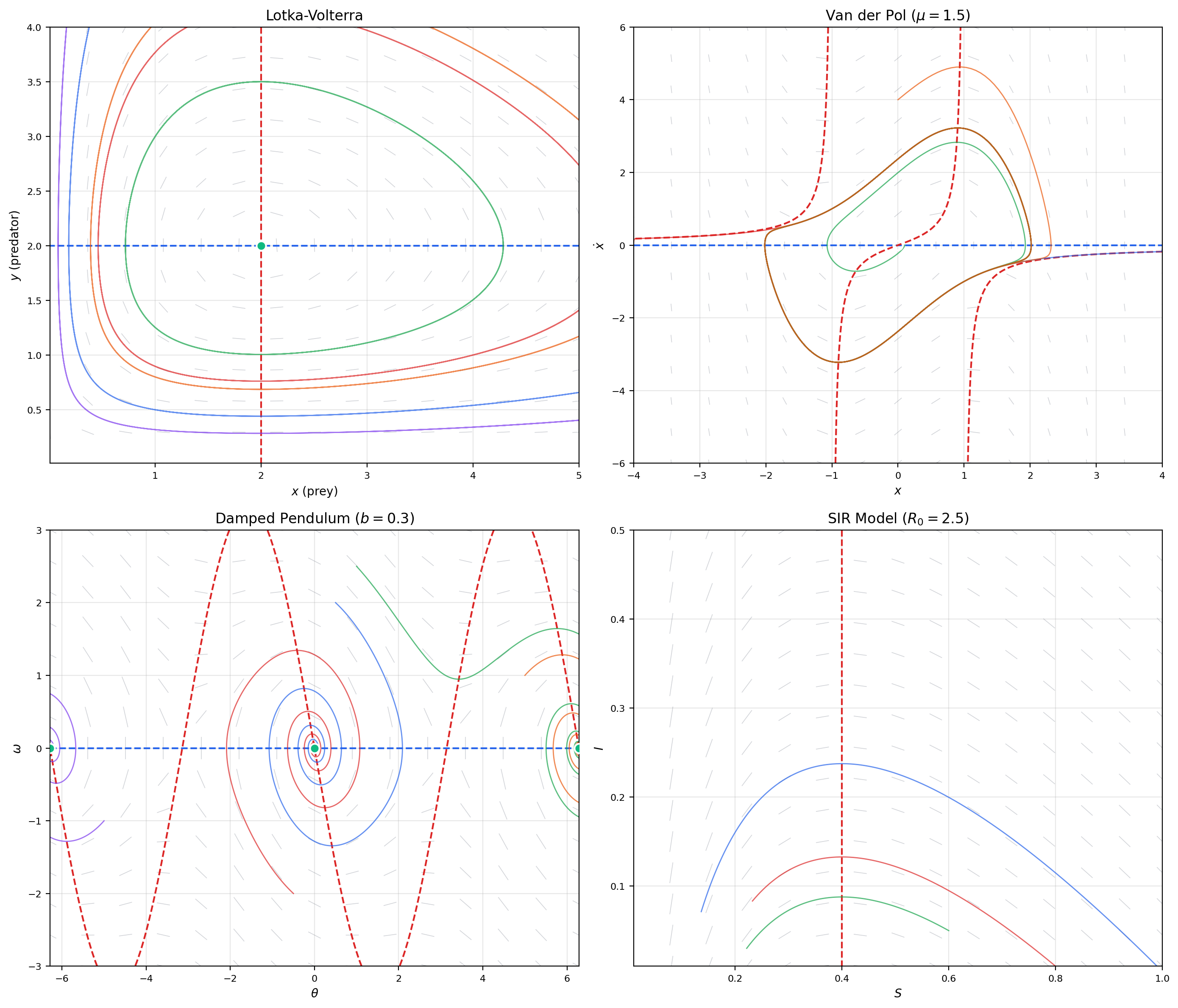
📝 Example 13 (Lotka-Volterra — Full Analysis)
The predator-prey system , with standard parameters :
- Equilibria: (saddle) and (center in linearization).
- Nullclines: or (x-nullcline); or (y-nullcline).
- Conserved quantity: is constant along trajectories. The orbits are closed curves — genuine periodic oscillations of predator and prey populations.
- Key feature: The nonzero equilibrium is a center, not merely in the linearization but in the full nonlinear system. This is exceptional — it relies on the special structure (Hamiltonian system). Generic perturbations break the closed orbits into spirals.
📝 Example 14 (Damped Pendulum — Separatrices)
The damped pendulum , with :
- Equilibria: . Even multiples of are stable spirals (downward rest positions); odd multiples are saddle points (upward balance points).
- Separatrices: The stable and unstable manifolds of the saddle points form heteroclinic connections — curves connecting one saddle to the next. These separatrices divide the phase plane into basins of attraction for the different stable equilibria.
- Physical interpretation: A trajectory starting with just enough energy to pass over the top of the pendulum follows a separatrix. Slightly less energy and it oscillates back; slightly more and it whips over the top and settles into the next well.
📝 Example 15 (SIR Epidemic Model)
The SIR model , models an epidemic:
- Equilibria: The line consists entirely of equilibria (disease-free states). The -nullcline divides the positive quadrant.
- Basic reproduction number: where is the initial susceptible fraction. If , the infected population initially grows (epidemic). If , it decays (no epidemic).
- Threshold behavior: This is a transcritical-type bifurcation in disguise. As decreases below during the epidemic, changes sign — the epidemic peaks and begins to decline. The parameter plays the role of the bifurcation parameter.
💡 Remark 8 (Gradient Systems — Always Stable, No Limit Cycles)
A gradient system uses itself as a Lyapunov function: . Consequences:
- Every trajectory converges to an equilibrium (no periodic orbits possible).
- Every local minimum of is an asymptotically stable equilibrium.
- Saddle points of have unstable manifolds of dimension equal to the Morse index (number of negative eigenvalues of ).
Gradient descent in ML is precisely a gradient system — which is why understanding loss landscape critical points is equivalent to stability analysis.
10. Computational Notes
Stability analysis in practice relies on numerical tools. Here are the key computational techniques.
Computing Jacobians. For an analytically given , symbolic differentiation is exact. For black-box systems (e.g., neural ODEs), use central finite differences: with (balancing truncation and roundoff error).
Solving the Lyapunov equation. In Python:
import numpy as np
from scipy.linalg import solve_continuous_lyapunov

A = np.array([[-1, 2], [-3, -2]])
Q = np.eye(2)
P = solve_continuous_lyapunov(A.T, -Q)  # Solves A^T P + P A = -Q
print("P =", P)
print("Eigenvalues of P:", np.linalg.eigvalsh(P))  # Should be positive
Continuation methods. Bifurcation diagrams are computed by continuation: start at a known equilibrium, then incrementally change while tracking the equilibrium position using Newton’s method. When the Jacobian becomes singular (a saddle-node) or eigenvalues cross the imaginary axis (a Hopf), the continuation algorithm detects the bifurcation. Software: AUTO, PyDSTool, MATCONT.
Lyapunov function construction via SDP. For polynomial systems, the search for a polynomial Lyapunov function can be cast as a semidefinite program (SDP): find such that satisfies , where is a vector of monomials. Tools like SOSTOOLS (MATLAB) and DSOS/SDSOS (Julia) automate this.
11. Connections to Statistics
MCMC ergodicity as dynamical-systems stability
Ergodicity of a Markov chain — convergence of the chain to its stationary distribution regardless of starting point — is the discrete-time analog of global stability of a dynamical system. Spectral gap analysis (second-largest eigenvalue of the transition operator) mirrors linear stability analysis of ODE equilibria. Lyapunov-function arguments for chain stability are the same arguments used here, transposed from continuous to discrete time. See formalStatistics Bayesian Computation & MCMC.
12. Connections to ML — Stability of Learning
The stability theory developed in this topic is the mathematical language of optimization dynamics. Here we make the connections explicit.
Loss landscape stability. A critical point of (where ) is the equilibrium of the gradient flow . The Jacobian of the RHS at is , so:
- Local minimum (): asymptotically stable. Gradient descent converges.
- Saddle point ( indefinite): unstable. The unstable manifold directions are the eigenvectors of with negative eigenvalues — these are the escape routes.
- Local maximum (): unstable in all directions.
In high dimensions (thousands of parameters), saddle points vastly outnumber local minima. The empirical observation that SGD reliably finds good minima is explained by the noise-driven escape from saddle points along the unstable manifold.
📝 Example 16 (Gradient Flow on a Loss Landscape with a Saddle Point)
Consider with critical point at the origin.
The gradient flow is , . The Hessian is — indefinite.
- Stable manifold : the -axis. Starting on , the -component decays and stays at zero. The iterate approaches the saddle.
- Unstable manifold : the -axis. Starting on , the -component grows exponentially. The iterate escapes the saddle.
In practice, SGD adds noise that has a component along , causing the iterate to escape the saddle point — this is the mechanism behind saddle-point escape in deep learning optimization.
GAN training dynamics. A GAN trains a generator and discriminator simultaneously. In simplified models, the training dynamics form a 2D system:
This is not a gradient system — it’s a saddle-point optimization (min-max). The Jacobian at equilibrium has the form , and its eigenvalues can be complex, leading to oscillatory behavior. Mode collapse corresponds to a bifurcation: as the generator becomes too confident, the equilibrium loses stability (a Hopf-like bifurcation) and training oscillates.
📝 Example 17 (Simplified GAN Dynamics)
Consider the simplified GAN: , where represents the generator and the discriminator.
The equilibrium at has Jacobian with eigenvalues — a center. The linearization predicts perpetual oscillation, and indeed the nonlinear system has a conserved quantity .
Adding regularization (spectral normalization of , gradient penalties) modifies the Jacobian to have — turning the center into a stable spiral and stabilizing training.
💡 Remark 9 (Learning Rate Schedules and Stability)
Stability theory explains why learning rate schedules work. Discrete gradient descent is a discretization of the gradient flow with step size . The discrete system is stable (converges) only if — the CFL-like condition for gradient descent.
A constant learning rate must satisfy everywhere along the trajectory. A learning rate schedule that decreases over time allows initially large steps (fast exploration, saddle escape via effective noise) that later shrink to ensure convergence (stability near the minimum). The schedule effectively transitions from the unstable regime (escape saddles) to the stable regime (converge to minimum).
13. Closing Reflection — The Qualitative Peak
This topic is the theoretical peak of the ODE track — the point where linear algebra (eigenvalues, matrix exponential) becomes predictive for nonlinear systems through linearization, and where energy methods (Lyapunov functions) provide an alternative path that doesn’t require solving the ODE.
Connections & Further Reading
Prerequisites — topics you need first
Linear Systems & Matrix Exponential
Phase portrait classification and eigenvalue methods from linear systems are the foundation of linearization stability analysis. The trace-determinant classification carries directly into the nonlinear Jacobian analysis.
The Hessian & Second-Order Analysis
Lyapunov functions use positive-definiteness criteria from Hessian analysis. The loss landscape Hessian eigenvalues determine gradient descent stability at critical points.
The Jacobian & Multivariate Chain Rule
Linearization computes the Jacobian of the vector field at an equilibrium. The Jacobian matrix is the system matrix A of the linearized system.
Partial Derivatives & the Gradient
Gradient systems y' = -∇V(y) are automatically stable with Lyapunov function V. The gradient provides the connection between scalar energy and vector dynamics.
First-Order ODEs & Existence Theorems
Existence and uniqueness (Picard-Lindelöf) guarantee that trajectories exist near equilibria and never cross — the foundation of qualitative analysis.
Inverse & Implicit Function Theorems
The Implicit Function Theorem determines when equilibria persist under parameter perturbation — the starting point of bifurcation theory.
Where this leads — next in formalCalculus
On to formalStatistics — where this calculus powers inference
On to formalML — where this calculus powers ML
Gradient Descent
Convergence of gradient descent to a local minimum is asymptotic stability of the gradient flow ODE. The Hessian eigenvalues at a critical point determine whether GD converges (stable) or diverges (unstable). Saddle-point escape is exit along the unstable manifold.
Information Geometry
Natural gradient descent stability depends on the eigenvalues of the preconditioned Hessian F⁻¹∇²L, where the Fisher metric reshapes the convergence landscape.
Smooth Manifolds
Stable and unstable manifolds of equilibria are immersed submanifolds. The Poincaré-Bendixson theorem extends to compact 2-manifolds. Dynamical systems on manifolds generalize phase portraits to curved spaces.
Spectral Theorem
The Lyapunov equation A^T P + PA = -Q is a Sylvester equation whose solvability depends on the spectra of A and -A^T. The spectral theorem guarantees P is symmetric positive-definite when A is Hurwitz.
References
- book Strogatz (2015). Nonlinear Dynamics and Chaos Chapters 5–8: stability, phase portraits, bifurcations, limit cycles. The primary reference for exposition style.
- book Perko (2001). Differential Equations and Dynamical Systems Chapters 2–3: linearization, Lyapunov stability, stable manifold theorem. More rigorous proofs.
- book Teschl (2012). Ordinary Differential Equations Chapters 6–7: stability theory, Poincaré-Bendixson theorem.
- paper Dauphin, Pascanu, Gulcehre, Cho, Ganguli & Bengio (2014). “Identifying and attacking the saddle point problem in high-dimensional non-convex optimization” Connects Hessian eigenvalue analysis to saddle point escape in deep learning — the stability theory of loss landscapes.