Partial Derivatives & the Gradient
Extending differentiation to functions of several variables — partial derivatives as single-variable slices, the gradient as the direction of steepest ascent, directional derivatives, and the total derivative as the correct notion of multivariable differentiability
Abstract. Partial derivatives extend single-variable differentiation to functions of several variables. Given f: ℝⁿ → ℝ, the partial derivative ∂f/∂xᵢ at a point a is computed by holding all variables except xᵢ fixed and taking the ordinary derivative — it measures the rate of change of f in the xᵢ-direction. Geometrically, for f: ℝ² → ℝ, ∂f/∂x is the slope of the curve obtained by slicing the surface z = f(x,y) with the plane y = a₂. Assembling all partial derivatives into a vector gives the gradient ∇f(a) = (∂f/∂x₁, ..., ∂f/∂xₙ). The gradient connects to directional derivatives via D_u f(a) = ∇f(a) · u: the rate of change of f in direction u is the dot product of the gradient with u. Since |∇f · u| ≤ ‖∇f‖ with equality when u = ∇f/‖∇f‖, the gradient points in the direction of steepest ascent, and its magnitude is the maximum rate of change. This is why gradient descent works: moving in the direction −∇L(θ) decreases the loss as rapidly as possible (locally). The gradient is perpendicular to level sets — contour lines on a topographic map run at right angles to the direction of steepest climb. But partial derivatives alone do not tell the whole story. The function f(x,y) = xy/(x² + y²) has both partial derivatives at the origin, yet is not even continuous there. The correct notion of differentiability in ℝⁿ is the total derivative: a linear map Df(a) satisfying lim_{h→0} |f(a+h) − f(a) − Df(a)·h| / ‖h‖ = 0. When f is differentiable, the total derivative is represented by the gradient (for scalar-valued f) or the Jacobian matrix (for vector-valued f, covered in the next topic). A sufficient condition for differentiability is that all partial derivatives exist and are continuous — the C¹ criterion. In machine learning, the gradient is the engine of optimization: SGD, Adam, and every gradient-based optimizer compute ∇L(θ) and step in the direction −∇L. Gradient magnitude |∂L/∂xᵢ| measures feature importance, saliency maps visualize which input pixels matter most to a classifier, and the geometry of loss landscapes — contour shapes, saddle points, local minima — is understood through the gradient and its higher-order relatives.
Overview & Motivation
In single-variable calculus, a function has one input and one direction to differentiate. The derivative captures everything about the local behavior of near : the rate of change, the tangent slope, the best linear approximation. We built that theory carefully in The Derivative & Chain Rule.
But a neural network’s loss depends on thousands or millions of parameters. To minimize , we need to know how changes when we nudge each parameter independently — that is a partial derivative — and then assemble those rates of change into a single direction for the next step — that is the gradient. The gradient tells us the direction of steepest ascent; negating it gives steepest descent; and the update rule is gradient descent.
This topic builds the theory that makes gradient-based optimization precise. We start with the geometric picture — slicing surfaces to extract ordinary derivatives — then assemble partial derivatives into the gradient, connect the gradient to directional derivatives and level sets, and confront the subtle question of what “differentiable” really means in .
Partial Derivatives
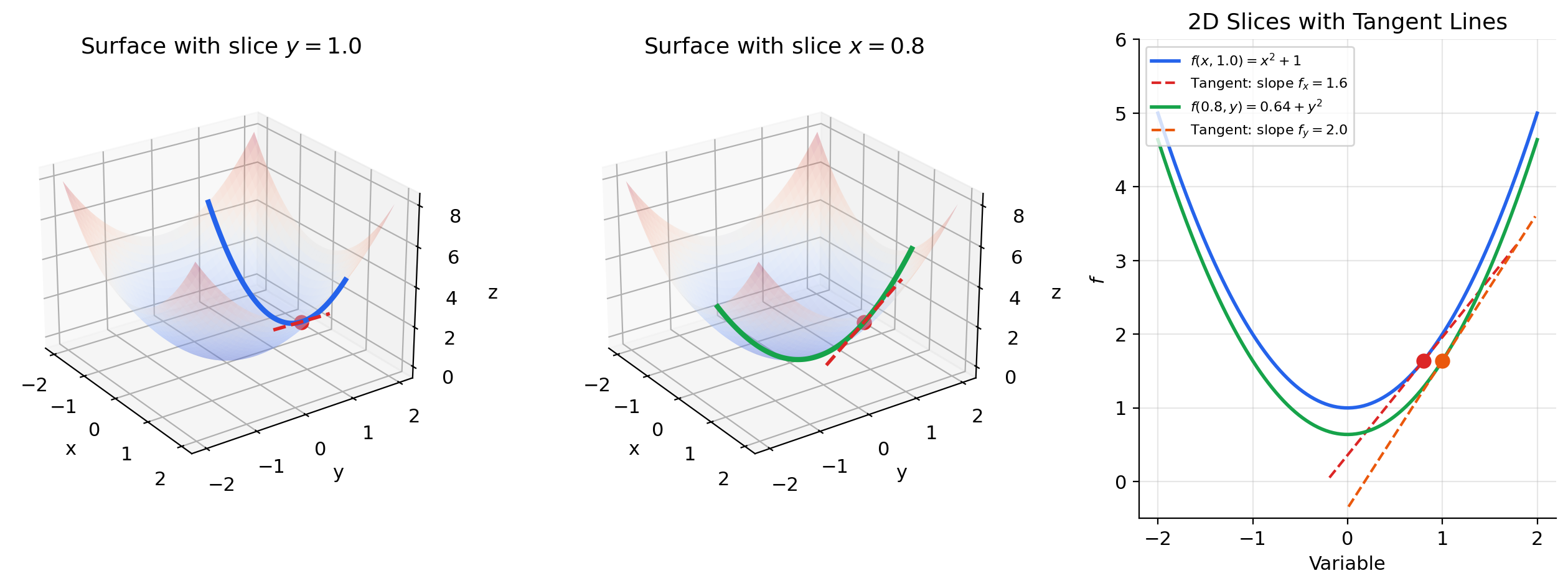
We begin with the simplest multivariable setup: a function , which we can visualize as a surface in three-dimensional space. To compute the partial derivative at a point , we slice the surface with the plane . This slice produces a curve in the -plane — an ordinary single-variable function of . The slope of this curve at is the partial derivative .
The key idea: a partial derivative is just an ordinary derivative, with all other variables held fixed.
📐 Definition 1 (Partial Derivative)
Let and let . The partial derivative of with respect to at is
provided this limit exists. In plain English: hold every input fixed except , and take the ordinary derivative with respect to .
Notation: .
This is exactly the limit definition of the derivative from The Derivative & Chain Rule, applied to the single-variable function .
📝 Example 1 (Partial derivatives of f(x,y) = x²y + sin(y))
To compute : treat as a constant and differentiate with respect to .
To compute : treat as a constant and differentiate with respect to .
At the point : and .
📝 Example 2 (Partial derivatives of f(x,y) = e^{x² + y²})
The chain rule from Topic 5 applies directly. Treating as constant:
Treating as constant:
At any point, and have the same exponential factor — they differ only in the leading coefficient ( vs. ). This symmetry reflects the rotational structure of .
Tangent Planes & Linear Approximation
In The Derivative & Chain Rule, the tangent line was the best linear approximation to near . In two variables, the tangent line becomes a tangent plane.
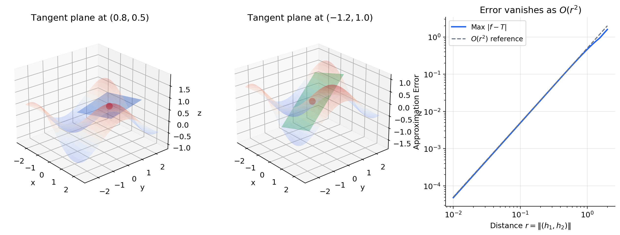
🔷 Proposition 1 (Tangent Plane as Linear Approximation)
If is differentiable at , then
with error that vanishes faster than as . The surface is the tangent plane to at .
The tangent plane touches the surface at one point and “hugs” it locally — just as the tangent line does in one dimension. Each partial derivative contributes one slope: is the slope in the -direction, is the slope in the -direction, and together they tilt the plane to match the surface.
💡 Remark 1 (From tangent line to tangent plane to tangent hyperplane)
In , the best linear approximation is a line. In , it is a plane. In , it is a hyperplane:
The pattern is the same — the derivative provides the coefficients of the linear approximation. In the next topic (The Jacobian & Multivariate Chain Rule), the derivative of a vector-valued function becomes a matrix, and the tangent hyperplane becomes an affine subspace.
The Gradient Vector
The individual partial derivatives tell us rates of change along coordinate directions. But there is nothing special about the coordinate axes — they are an arbitrary choice of basis for . The gradient collects all partial derivatives into a single vector that encodes the rate of change in every direction simultaneously.
📐 Definition 2 (The Gradient)
Let be a function whose partial derivatives all exist at . The gradient of at is the vector
Notation: . We follow the column-vector convention throughout: is a column vector in .
The gradient transforms the partial derivative — a collection of separate numbers — into a single geometric object: a vector that lives in the same space as the input. This shift from “list of rates” to “direction in input space” is the conceptual leap that makes gradient-based optimization geometric.
📝 Example 3 (Gradient of f(x,y) = x² + y²)
At any point, the gradient points radially outward from the origin — directly “uphill” on the paraboloid. At : , pointing toward the northeast. The magnitude measures how steep the surface is at that point.
📝 Example 4 (Gradient of f(x,y,z) = xyz)
At : . The function is most sensitive to changes in (rate ), less sensitive to (rate ), and least sensitive to (rate ). In an ML context, this is feature importance: the gradient magnitude per coordinate tells you which inputs matter most.
Directional Derivatives
Partial derivatives measure the rate of change along the coordinate axes . But we often need the rate of change in a direction that is not aligned with any axis — for instance, the direction a gradient descent step actually takes.
📐 Definition 3 (Directional Derivative)
Let , , and a unit vector (). The directional derivative of at in the direction is
provided this limit exists. In plain English: stand at , walk in direction , and measure how fast changes.
Notice that choosing (the -th standard basis vector) recovers the partial derivative . Partial derivatives are special cases of directional derivatives — the special cases where the direction is along a coordinate axis.
The remarkable fact is that when is differentiable, the directional derivative in any direction can be computed from the gradient alone:
🔷 Theorem 1 (Gradient–Directional Derivative Relationship)
If is differentiable at , then for every unit vector , the directional derivative exists and equals
Proof.
Define . This is a function — a single-variable function obtained by restricting to the line through in direction . By definition, .
Since is differentiable at , the chain rule (The Derivative & Chain Rule, Theorem 6) applies to the composition . The “inner function” is , with . The chain rule gives:
The chain rule is valid here because is differentiable at — not merely having partial derivatives. This distinction is critical and we return to it in Section 7. ∎
📝 Example 5 (Directional derivative of f(x,y) = x² + y² in direction u = (1,1)/√2)
At : . In the direction :
Compare this with the partial derivatives: and . The directional derivative in the diagonal direction is larger than either partial derivative individually — because the gradient points diagonally, and we are measuring rate of change in the gradient’s own direction.
The Gradient as Steepest Ascent
We now arrive at the geometric crown jewel of this topic: the gradient points in the direction of steepest ascent. This is why gradient descent works — it follows , which is the direction of steepest descent.
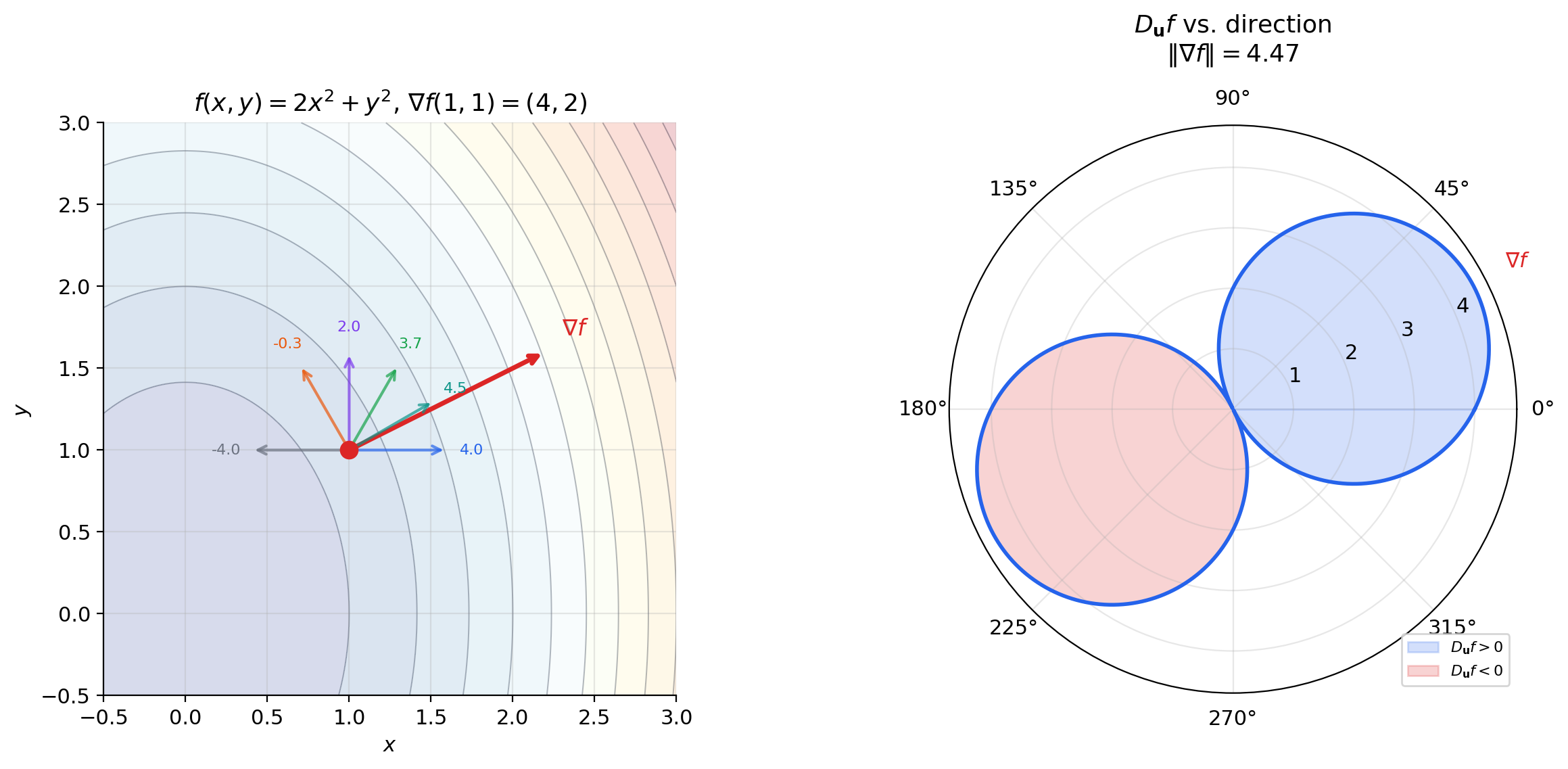
🔷 Theorem 2 (Gradient as Direction of Steepest Ascent)
Let be differentiable at with . Then among all unit vectors :
- The maximum of is , achieved when .
- The minimum of is , achieved when .
- if and only if is orthogonal to .
Proof.
By Theorem 1, . By the Cauchy-Schwarz inequality:
since . Equality holds if and only if is a scalar multiple of . Since , this means .
The positive sign gives (the maximum). The negative sign gives (the minimum). If , then . ∎
This theorem has an immediate and profound consequence for optimization: to decrease as fast as possible from the current point , walk in the direction . The maximum rate of decrease is . No other direction does better.
The gradient is not merely “some direction of increase” — it is the unique optimal direction, and its magnitude tells you the maximum possible rate of change. Directions perpendicular to the gradient produce zero change — they trace out the level set.
🔷 Theorem 3 (Gradient is Orthogonal to Level Sets)
Let be differentiable at with . Let be the level set through . If is a smooth curve with and for all , then
In words: the gradient is perpendicular to every curve that stays on the level set.
Proof.
Since for all (the curve stays on the level set), differentiating with respect to at gives:
by the chain rule. This holds for every tangent vector to at , so is orthogonal to the tangent space of at . ∎
💡 Remark 2 (Contour maps and topographic intuition)
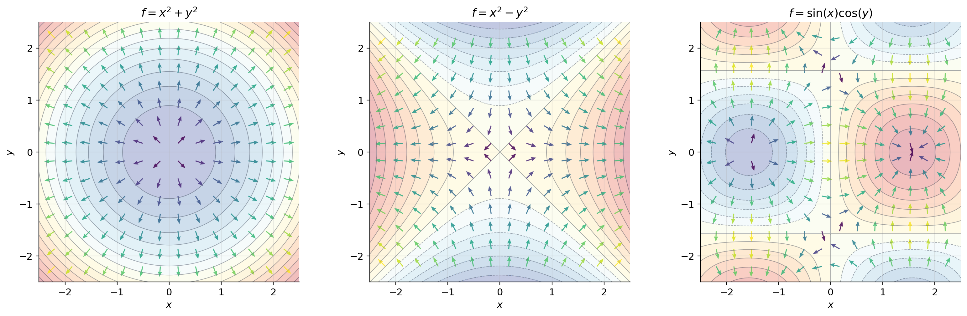
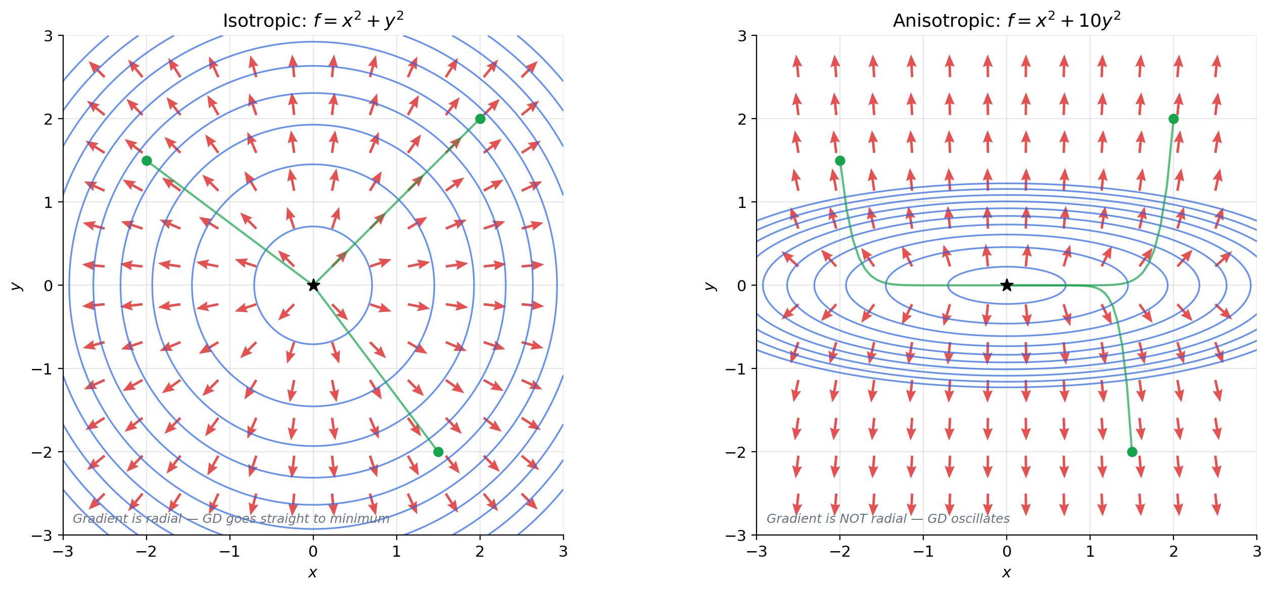
On a topographic map, contour lines connect points at the same elevation. The gradient points in the direction of steepest climb — straight up the hillside, perpendicular to the contour lines. A hiker following the gradient path reaches the summit as fast as possible; a hiker walking along a contour line (perpendicular to the gradient) stays at the same elevation. Gradient descent reverses this: it follows , going downhill as steeply as possible.
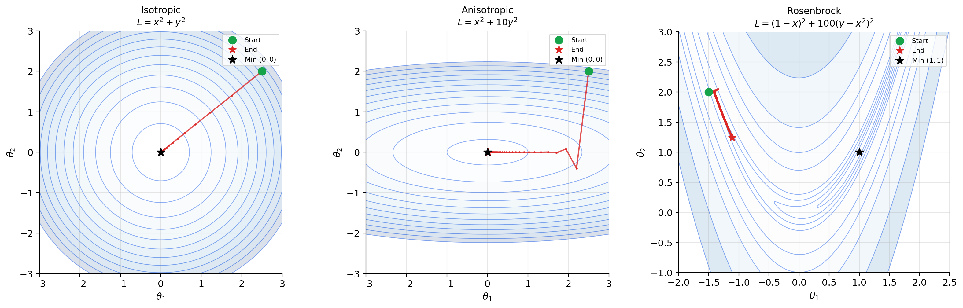
For a loss function with circular contours (isotropic loss, like ), the gradient points radially inward and gradient descent takes a straight path to the minimum. For elongated contours (anisotropic loss, like ), the gradient does not point toward the minimum — it points perpendicular to the contour, which may oscillate back and forth across the narrow valley. This is exactly why momentum and adaptive methods like Adam were invented.
Differentiability in — The Total Derivative
We have been using the word “differentiable” in our theorems, and it is time to be precise about what it means. In single-variable calculus, differentiability meant that the limit exists. The multivariable situation is more subtle.
The subtle point: having all partial derivatives is not the same as being differentiable. Partial derivatives probe a function only along coordinate axes — a set of rays emanating from . A function can have well-defined partial derivatives at a point but behave wildly when approached from other directions. The correct notion of differentiability requires the function to be well-approximated by a single linear map in all directions simultaneously.
📐 Definition 4 (Differentiability (Total Derivative))
A function is differentiable at if there exists a linear map such that
When is differentiable, is unique and is represented by the gradient: . For , is represented by the Jacobian matrix — that is the next topic.
The limit says: the linear approximation matches so well that the error shrinks faster than itself. Compare this with the single-variable case from The Derivative & Chain Rule: . The multivariable version is the same idea, but the limit is in — the approach direction is unrestricted.
🔷 Theorem 4 (Differentiability Implies Partial Derivatives Exist)
If is differentiable at , then all partial derivatives exist at , and .
Proof.
Set (approach along the -th coordinate axis) in the total derivative definition:
Since is linear, . Rearranging:
The left side of the subtraction is exactly the difference quotient defining . So the partial derivative exists and equals . ∎
💡 Remark 3 (The converse is false)
Partial derivatives existing does not imply differentiability. This echoes the single-variable situation (continuity does not imply differentiability), but in a stronger form: in , we can have all partial derivatives at a point and still fail to be continuous there. The following example demonstrates this dramatically.
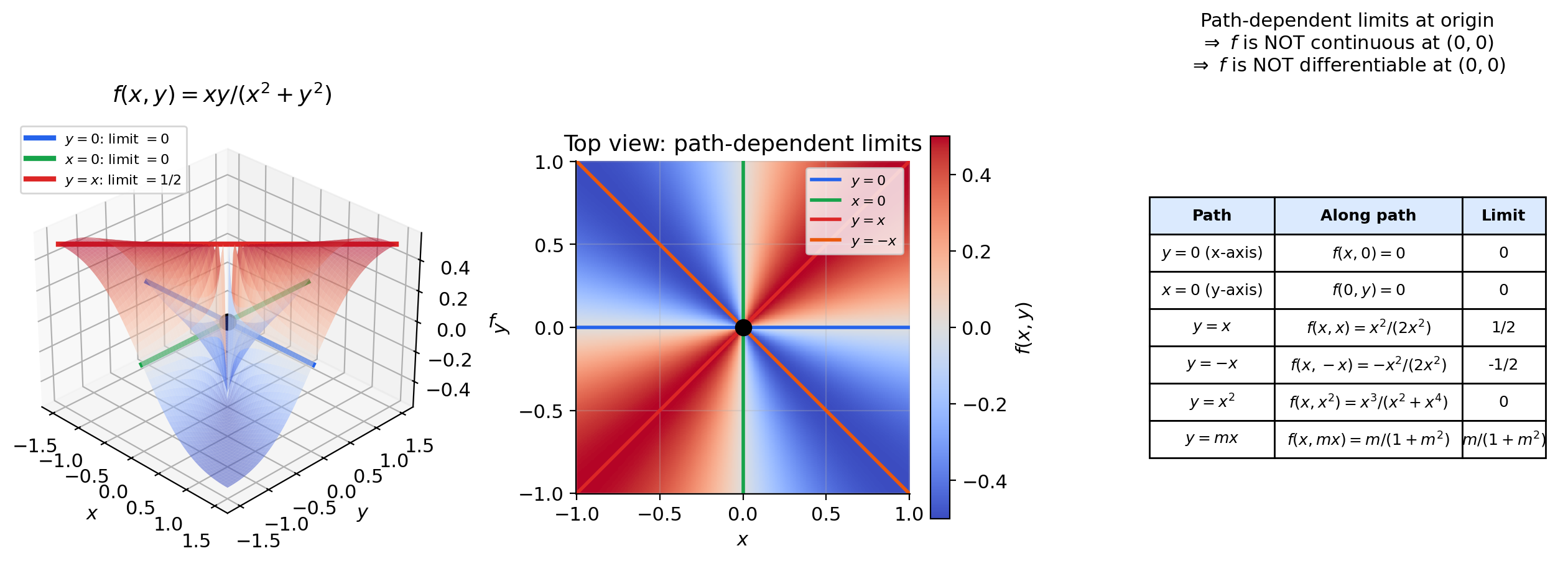
📝 Example 6 (The critical counterexample)
Define
Partial derivatives at the origin exist and equal zero:
Similarly . Both partial derivatives exist because along the coordinate axes, is identically zero.
But is not continuous at the origin: Along the line ,
The function approaches along the diagonal but equals at the origin. Since is not continuous, it certainly cannot be differentiable — yet both partial derivatives exist. The moral: partial derivatives probe only the coordinate directions; differentiability requires consistent behavior from all directions simultaneously.
The positive result — a sufficient condition for differentiability — requires the partial derivatives to be continuous, not merely to exist:
🔷 Theorem 5 (C¹ Criterion)
If all partial derivatives exist in a neighborhood of and are continuous at , then is differentiable at .
Proof.
We sketch the proof for ; the general case is analogous. Write:
Apply the single-variable Mean Value Theorem (Mean Value Theorem & Taylor Expansion, Theorem 1) to each bracket:
- The first bracket equals for some between and .
- The second bracket equals for some between and .
So:
Now subtract the linear approximation :
By continuity of and at : as , we have and , so and . Call these differences and , both tending to zero. Then:
Dividing by : the error ratio is at most . ∎
💡 Remark 4 (Differentiability implies continuity (the chain of implications))
Just as in The Derivative & Chain Rule, differentiability at implies continuity at :
The chain of implications is:
but none of the converses hold in general. The criterion is the practical workhorse: in virtually every function arising in machine learning (polynomials, exponentials, compositions of smooth functions), the partial derivatives are continuous, so differentiability is automatic.
Computational Notes
Computing gradients is the central computational task in gradient-based optimization. There are three approaches:
Analytical gradients. When we know the formula for , we compute by hand (or symbolically). For , the gradient is — exact, fast, no approximation error. This is always preferred when available.
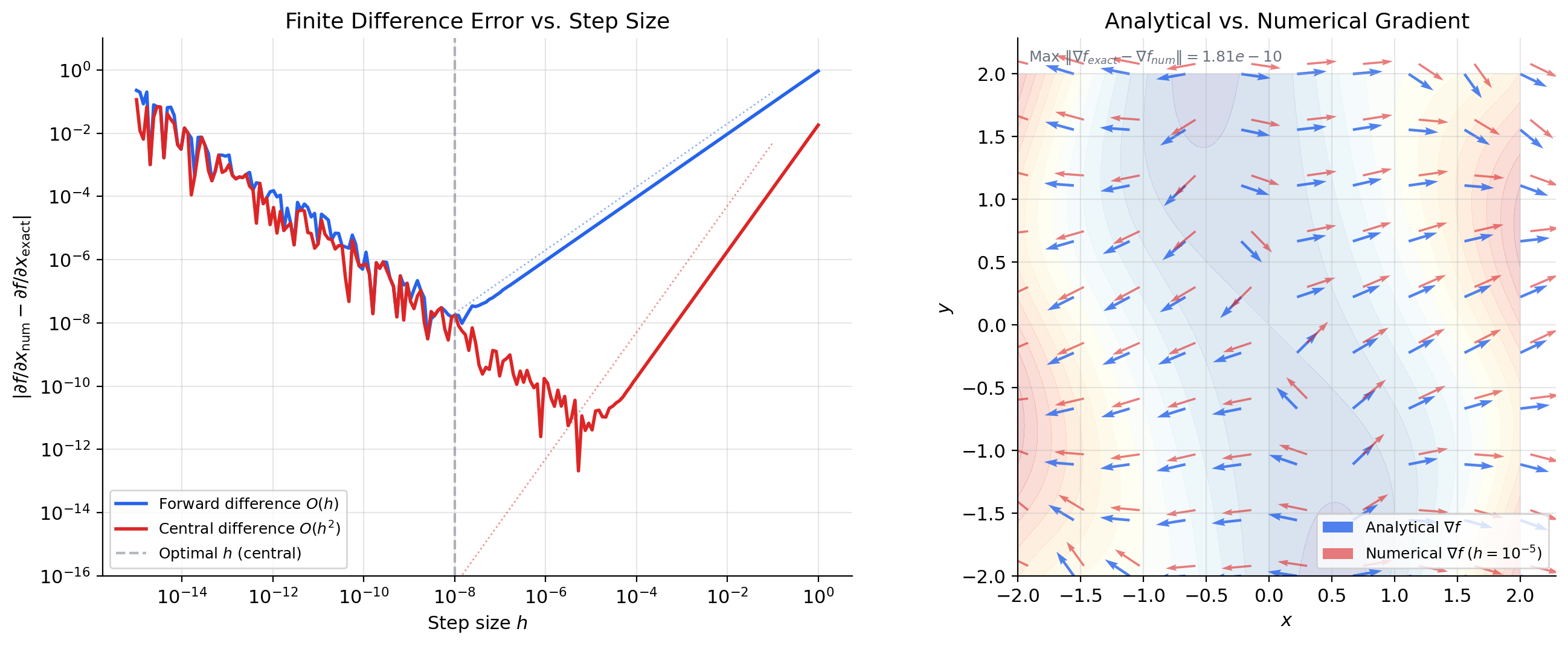
Finite difference gradients. When we don’t have a formula (or want to verify one), we approximate each partial derivative numerically:
This is the same central difference from The Derivative & Chain Rule, applied coordinate by coordinate. The tradeoff is the same: too large gives truncation error; too small gives floating-point cancellation error. For variables, we need function evaluations — one forward and one backward per coordinate.
In Python, scipy.optimize.approx_fprime(x, f, epsilon) computes the finite-difference gradient. NumPy’s numpy.gradient handles gridded data.
Automatic differentiation. The jax.grad function computes exact gradients (to machine precision) without finite differences, using reverse-mode automatic differentiation — the same algorithm as backpropagation. A preview:
import jax
import jax.numpy as jnp

f = lambda x: x[0]**2 + x[1]**2
grad_f = jax.grad(f)
grad_f(jnp.array([1.0, 1.0]))  # → [2.0, 2.0]
This computes the exact gradient at cost proportional to a single function evaluation, regardless of the number of variables . Automatic differentiation is the computational backbone of modern deep learning — we will see how it works in detail when we reach the Jacobian and the multivariate chain rule.
Connections to Statistics
The gradient is the engine behind almost every estimator and sampler in modern statistics. Score functions, Newton/IRLS updates, HMC dynamics, ridge/lasso optimality conditions — all of them are gradient operations.
Maximum likelihood
The score vector is the gradient of the log-likelihood. Gradient ascent on the log-likelihood, the geometry of the likelihood surface, and the steepest-ascent interpretation all apply directly to MLE. See formalStatistics Maximum Likelihood.
HMC and Langevin dynamics
Hamiltonian Monte Carlo and the No-U-Turn Sampler require evaluating at every leapfrog step. Langevin MCMC uses the gradient of the log-density as a drift term. Gradient availability is the practical distinction between HMC and random-walk Metropolis. See formalStatistics Bayesian Computation & MCMC.
GLMs and penalized regression
The IRLS algorithm for fitting generalized linear models is Newton’s method on the gradient of the log-likelihood. Ridge and lasso are problems — penalized gradient equations. See formalStatistics Generalized Linear Models and formalStatistics Regularization & Penalized Estimation.
Connections to ML
The gradient is the most operationally important object in machine learning optimization. Every concept in this topic has a direct counterpart in ML practice.
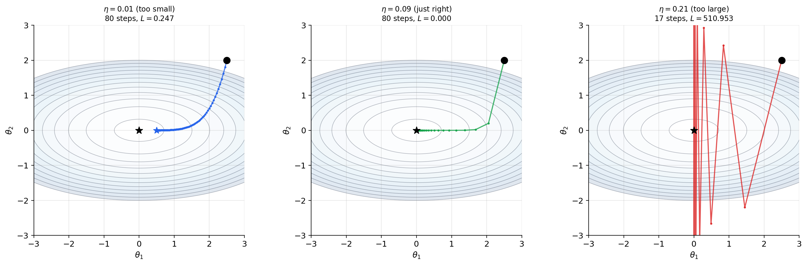
Gradient descent. The update rule is the literal definition of gradient descent: evaluate the gradient of the loss, step in the opposite direction (steepest descent), and repeat. The learning rate controls the step size. Theorem 2 explains why this is locally optimal: no other direction decreases faster than .
Loss landscape geometry. The geometry of the loss function determines how gradient descent behaves. Contour plots reveal this geometry: circular contours (isotropic loss) mean gradient descent takes a direct path to the minimum. Elongated contours (anisotropic loss) mean gradient descent oscillates — the gradient perpendicularity to contour lines (Theorem 3) causes the path to zig-zag across the narrow valley. This oscillation motivates momentum, RMSProp, and Adam, which adapt the effective learning rate per coordinate. Second-order methods using the Hessian (The Hessian & Second-Order Analysis) address this more directly.
Feature importance and saliency. The magnitude measures how sensitive the loss is to feature . If is large while is small, then feature has more influence on the prediction. In deep learning, saliency maps compute to visualize which pixels most affect the classifier’s output — a direct application of partial derivatives.
Critical points. A critical point has : the loss surface is flat. But does not distinguish minima from maxima from saddle points — that requires the Hessian (the matrix of second-order partial derivatives, covered in The Hessian & Second-Order Analysis). In high-dimensional loss landscapes, saddle points are far more common than local minima, and the gradient alone cannot tell them apart.
Connections & Further Reading
Prerequisites — topics you need first
The Derivative & Chain Rule
Partial derivatives are single-variable derivatives in disguise: hold all variables except one fixed and apply the limit definition from Topic 5. Every concept here — the limit definition, differentiability vs. continuity, linear approximation — is the multivariable extension of its Topic 5 counterpart.
Epsilon-Delta & Continuity
The total derivative definition uses a multivariable limit (‖h‖ → 0 in ℝⁿ), extending the ε-δ framework from Topic 2 to higher dimensions. The C¹ criterion uses continuity of partial derivatives, also in the ε-δ sense.
Completeness & Compactness
Compactness of closed bounded sets in ℝⁿ (Heine-Borel generalizes) ensures that continuous functions on compact domains achieve extrema — the multivariable Extreme Value Theorem that motivates gradient-based search for minima.
Where this leads — next in formalCalculus
On to formalStatistics — where this calculus powers inference
Maximum Likelihood
The score vector U(θ) = ∇_θ log L is the gradient of the log-likelihood. Gradient ascent on the log-likelihood, the geometry of the likelihood surface, and the steepest-ascent interpretation all apply directly to MLE.
Bayesian Computation And MCMC
Hamiltonian Monte Carlo (HMC) and the No-U-Turn Sampler require evaluating ∇_θ log p(θ|x) at every leapfrog step. Langevin MCMC uses the gradient of the log-density as a drift term. Gradient availability is the practical distinction between HMC and random-walk Metropolis.
Generalized Linear Models
The IRLS algorithm for fitting GLMs is Newton's method on the gradient of the log-likelihood. The score ∇_β ℓ(β) and its Hessian are the engines of the fitting procedure.
Regularization And Penalized Estimation
Ridge and lasso are ∇_β L(β) + ∇_β P(β) = 0 problems — penalized gradient equations. Coordinate descent and proximal methods for lasso are all gradient-adjacent optimization schemes.
Hierarchical Bayes And Partial Pooling
Empirical-Bayes estimation of hyperparameters uses gradient-based optimization of the marginal likelihood. Full Bayes via HMC needs gradients of the hierarchical log-posterior, whose group-vs-individual structure shapes the geometry.
Bayesian Foundations And Prior Selection
Topic 25's Bernstein–von Mises proof (§25.8 Proof 3) Taylor-expands the log-posterior around θ̂_MLE in multiple dimensions — the leading Gaussian term comes from the first- and second-order terms of the multivariate expansion. Laplace approximation is multivariate Taylor with a Hessian determinant.
Model Selection And Information Criteria
Topic 24's AIC derivation (§24.3 Proof 1) Taylor-expands ℓ(θ) around θ_0 in (p+1) dimensions; the BIC-Laplace proof (§24.4 Proof 2) does multivariate Laplace with a Hessian determinant. Both rely on the second-order multivariate Taylor expansion developed here.
On to formalML — where this calculus powers ML
Gradient Descent
Gradient descent updates parameters by stepping in the direction −∇L(θ) — the steepest descent direction. The gradient's orthogonality to level sets explains why gradient descent cuts across contour lines. The directional derivative inequality D_u f ≤ ‖∇f‖ quantifies why no other direction decreases the loss faster (locally).
Convex Analysis
For convex functions, the gradient provides a global lower bound: f(y) ≥ f(x) + ∇f(x)ᵀ(y − x). This first-order convexity condition is the foundation of convex optimization — the gradient at any point gives a tangent hyperplane that lies entirely below the graph.
Smooth Manifolds
The gradient of a constraint function g is normal to the level set g⁻¹(c). This geometric fact — that ∇g is perpendicular to the constraint surface — is the starting point for Lagrange multipliers and the theory of smooth submanifolds of ℝⁿ.
Clustering
The clustering topic uses partial-derivative machinery for the mean-shift derivation (§3 chain rule on the KDE estimate ∇f̂_h) and the §4 convergence proof (multivariate Taylor expansion around a mode). Mode-seeking algorithms reduce to gradient ascent on the density estimate.
References
- book Abbott (2015). Understanding Analysis Single-variable foundation — Topic 5 of formalCalculus follows Abbott's Chapter 5. This topic extends that foundation to several variables.
- book Munkres (1991). Analysis on Manifolds Chapters 2–3 develop partial derivatives, the total derivative, and the chain rule in ℝⁿ with full rigor and exceptional clarity — the primary reference for our multivariable treatment
- book Rudin (1976). Principles of Mathematical Analysis Chapter 9 on multivariable differentiation — compact, definitive treatment of the total derivative and the inverse function theorem
- book Spivak (1965). Calculus on Manifolds Chapter 2 develops the derivative as a linear map, the multivariate chain rule, and partial derivatives — elegant minimalist treatment
- book Goodfellow, Bengio & Courville (2016). Deep Learning Section 4.3 on gradient-based optimization — the gradient as the engine of deep learning training
- paper Li, Xu, Taylor, Studer & Goldstein (2018). “Visualizing the Loss Landscape of Neural Nets” Loss landscape geometry — contour plots, saddle points, and the role of gradient direction in navigating high-dimensional optimization surfaces