Mean Value Theorem & Taylor Expansion
Local approximation theory — the theorems that connect a function's derivatives to its global behavior, and the polynomial approximations that power convergence analysis in optimization
Abstract. The Mean Value Theorem says that if f is continuous on [a,b] and differentiable on (a,b), there exists c ∈ (a,b) where f'(c) = [f(b) - f(a)]/(b - a) — the instantaneous rate of change at some interior point equals the average rate of change over the whole interval. Geometrically, this means every secant line has a parallel tangent line somewhere between the endpoints. This single theorem has sweeping consequences: it proves that functions with zero derivative are constant, that the sign of f' determines monotonicity, and that bounded derivatives imply Lipschitz continuity. The proof goes through Rolle's theorem — the special case where f(a) = f(b), so the guaranteed interior point is a local extremum with f'(c) = 0 — which itself depends on the Extreme Value Theorem from compactness. Taylor's theorem extends the Mean Value Theorem from first-order to arbitrary-order approximation: near any point a, a sufficiently smooth function is approximated by its degree-n Taylor polynomial Tₙ(x) = Σ f⁽ᵏ⁾(a)/k! (x - a)ᵏ, with the Lagrange remainder Rₙ = f⁽ⁿ⁺¹⁾(c)/(n+1)! (x - a)ⁿ⁺¹ providing a quantitative error bound. Taylor expansion is the analytical engine behind convergence rate proofs in optimization: the descent lemma f(y) ≤ f(x) + ∇f(x)ᵀ(y - x) + (L/2)‖y - x‖² is a second-order Taylor bound, and Newton's method achieves quadratic convergence by optimizing the local quadratic Taylor model at each step.
Overview & Motivation
You’re training a neural network and observe that the loss drops from to over 100 gradient descent steps. Can you guarantee that at some point during training, the loss was decreasing at a rate of exactly per step? The Mean Value Theorem says yes — and this kind of “existence of an intermediate rate” argument is exactly what convergence proofs exploit.
Moreover, how well can you approximate the loss near the current parameter? The tangent line approximation from The Derivative & Chain Rule gives a first-order answer: . But this approximation degrades as grows. Taylor expansion provides higher-order corrections — the second-order approximation is what Newton’s method uses, and the quality of these approximations determines whether your optimizer converges linearly or quadratically.
This topic develops both ideas rigorously. We start with Rolle’s theorem and the Mean Value Theorem — the existence results that connect local derivatives to global behavior — then build Taylor’s theorem, which extends linear approximation to polynomial approximation of arbitrary degree. The MVT earns its name through three sweeping consequences: zero derivative implies constant, derivative sign determines monotonicity, and bounded derivatives imply Lipschitz continuity. Taylor’s theorem earns its keep by powering every convergence rate proof in optimization.
Prerequisites: We use the derivative definition and differentiation rules from The Derivative & Chain Rule, and the Extreme Value Theorem from Completeness & Compactness — specifically, that a continuous function on a closed bounded interval achieves its maximum and minimum.
Rolle’s Theorem
The geometric picture
Imagine a continuous curve that starts and ends at the same height — say, you drive from home, travel some distance, and return to the same elevation. At some point during the trip, your altitude was neither increasing nor decreasing: you were at a turning point. In the language of calculus, there must be at least one point where the tangent to the curve is horizontal.
This is Rolle’s theorem in a sentence: if and is smooth enough in between, then for some interior point .
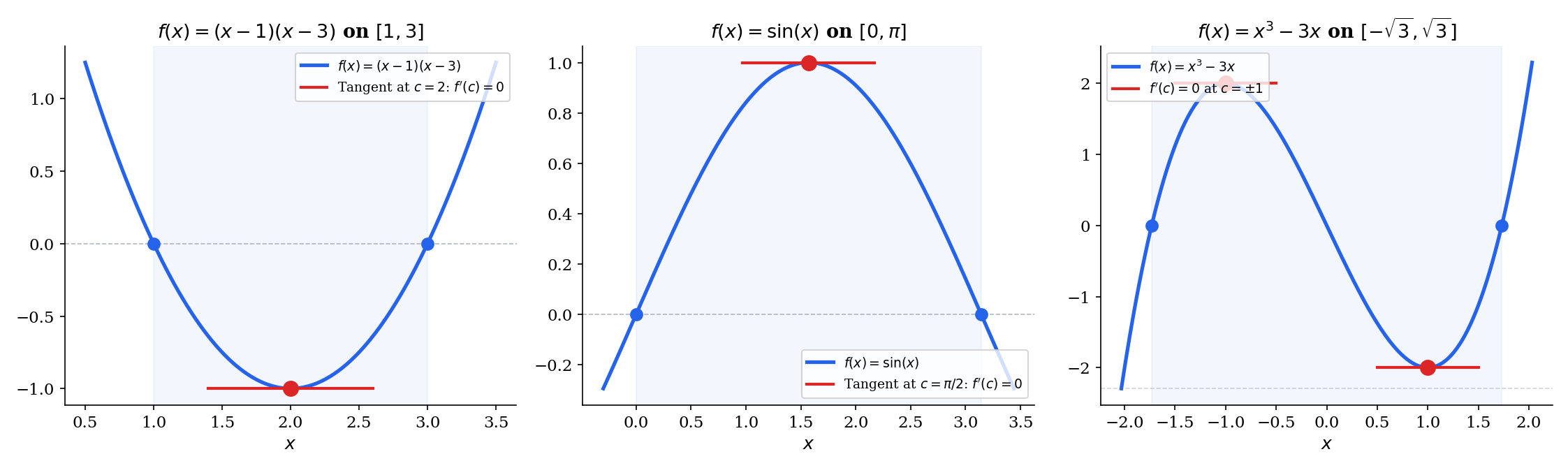
🔷 Theorem 1 (Rolle's Theorem)
Let be continuous on and differentiable on , with . Then there exists such that .
Proof.
By the Extreme Value Theorem — which we proved in Completeness & Compactness using the Heine-Borel theorem — the continuous function on the compact set achieves its maximum value and its minimum value .
Case 1: If , then is constant on , so for every .
Case 2: If , then since , at least one of or is achieved at an interior point (both endpoints have the same value, so if the max and the min were both at the endpoints, we’d have , contradicting ).
Without loss of generality, suppose with . Since is a local maximum and is differentiable at , we have:
- For sufficiently small: (since ), so .
- For sufficiently small: (since and ), so .
Together: .
📝 Example 1 (Rolle's on f(x) = x² − 4x + 3 on [1, 3])
We verify: and , so . The derivative is , which vanishes at . Geometrically, the parabola dips below the -axis and turns around at its vertex .
💡 Remark 1 (Why all three hypotheses matter)
Each hypothesis in Rolle’s theorem is essential — removing any one produces a counterexample:
(i) Not continuous: Define on by for and . Then , and is differentiable on with for all — so there is no with . The discontinuity at breaks Rolle’s conclusion.
(ii) Not differentiable: on has , but does not exist (the left and right derivatives disagree — we saw this in The Derivative & Chain Rule, Example 3). The minimum of is at , exactly where differentiability fails.
(iii) Not : The function on has everywhere. Without the equal-endpoint condition, there’s no reason to expect a horizontal tangent.
Try toggling “Break hypotheses” in the explorer below to see each failure mode.
The Mean Value Theorem
From horizontal to parallel
Rolle’s theorem requires — a strong condition. The Mean Value Theorem removes it. The key insight is geometric: tilt your head until the secant line connecting and is horizontal, and you’re back to Rolle’s setup. More precisely, subtract the secant line from , and the resulting function has equal endpoints.
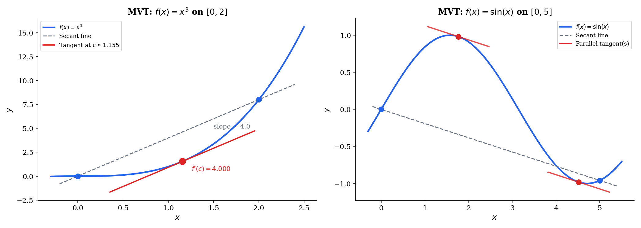
🔷 Theorem 2 (The Mean Value Theorem)
Let be continuous on and differentiable on . Then there exists such that
In words: the instantaneous rate of change at some interior point equals the average rate of change over .
Proof.
Define the auxiliary function
This is minus the secant line through and .
Check the hypotheses of Rolle’s theorem:
- is continuous on (difference of continuous functions).
- is differentiable on (difference of differentiable functions).
- and , so .
By Rolle’s theorem, there exists with . Since
we get .
The proof is a one-line reduction to Rolle’s theorem — but it’s the choice of the auxiliary function that makes it work. The idea is to subtract exactly the right linear function so that the endpoints align.
📝 Example 2 (MVT on f(x) = x³ on [0, 2])
The secant slope is . We need , so .
Drag the and sliders in the explorer below to see how the secant line and the parallel tangent change for different intervals.
Consequences of the Mean Value Theorem
The MVT is the bridge between local information (the derivative at a point) and global behavior (the function’s values over an interval). Three consequences demonstrate its power — and each one is a workhorse in analysis and optimization.
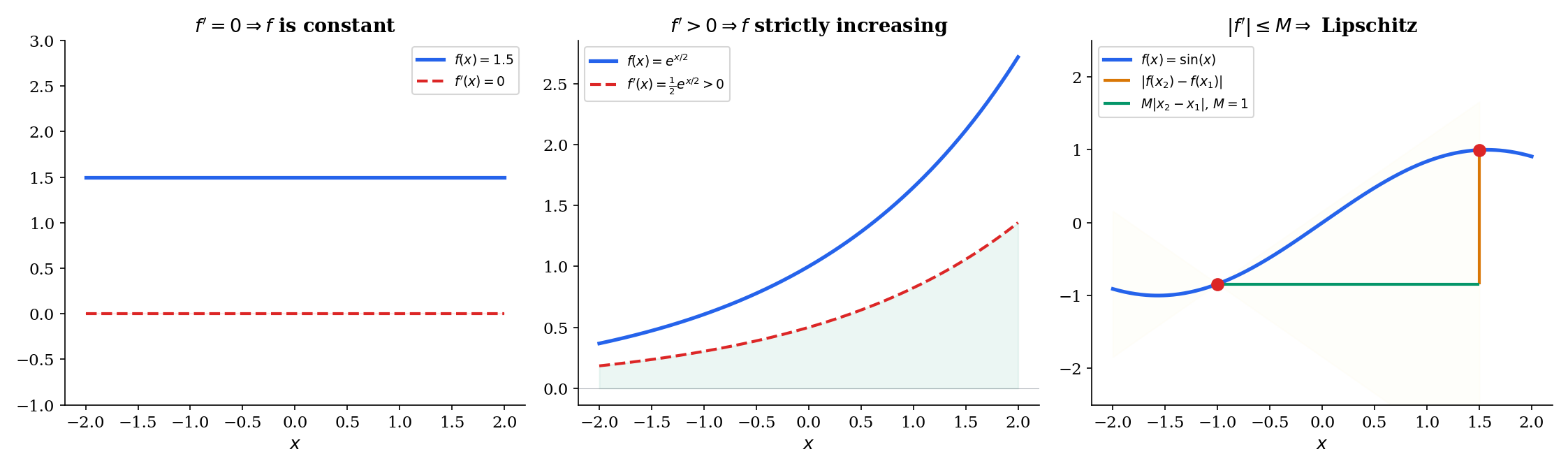
🔷 Corollary 1 (Zero Derivative Implies Constant)
If is differentiable on and for all , then is constant on .
Proof.
For any with , the MVT gives
for some . Hence for all .
🔷 Corollary 2 (Monotonicity from Derivative Sign)
Let be differentiable on .
- If for all , then is strictly increasing on .
- If for all , then is strictly decreasing on .
Proof.
Suppose on and take in . By the MVT, there exists with
Since and , we get , i.e., . The decreasing case is symmetric.
🔷 Corollary 3 (Bounded Derivative Implies Lipschitz)
If is differentiable on and for all , then
Proof.
By the MVT, .
💡 Remark 2 (Lipschitz continuity and ML)
The Lipschitz constant bounds how fast can change. In machine learning, the Lipschitz gradient condition is the single most important regularity assumption in convergence proofs for gradient descent. It comes directly from applying the MVT (or its multivariable analog) to : if exists and , then the gradient is -Lipschitz. This determines the maximum safe learning rate and the convergence rate for gradient descent on convex functions. (→ formalML: Gradient Descent)
Cauchy’s Mean Value Theorem and L’Hôpital’s Rule
The standard MVT compares to the identity function . Cauchy’s generalization compares two functions simultaneously.
🔷 Theorem 3 (Cauchy's Mean Value Theorem)
Let and be continuous on and differentiable on , with for all . Then there exists such that
Proof.
First note that (otherwise, Rolle’s theorem applied to would give for some , contradicting our hypothesis). Define
Then is continuous on , differentiable on , and . By Rolle’s theorem, there exists with :
Since and , dividing gives the result.
The standard MVT is the special case . The power of Cauchy’s version is that it lets us evaluate limits of ratios — which brings us to L’Hôpital’s Rule.
🔷 Theorem 4 (L'Hôpital's Rule (0/0 form))
Suppose and are differentiable near (except possibly at ), with near . If
and the limit exists (finite or ), then
Proof.
Define so that and are continuous at . For near with , Cauchy’s MVT on (or ) gives a point between and with
As , (squeezed between and ), so .
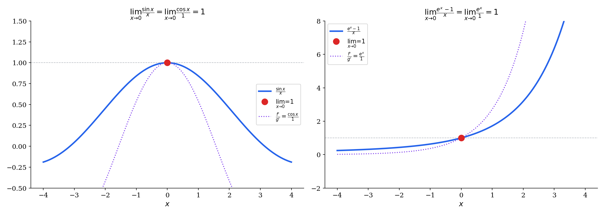
📝 Example 3 (L'Hôpital's applied: lim sin(x)/x)
is the form. Applying L’Hôpital’s:
We previously established this limit geometrically (a squeeze argument involving areas). Now we have a second, purely analytical proof via Cauchy’s MVT. Both proofs are valid; the geometric argument is more elementary, while L’Hôpital’s is more general.
💡 Remark 3 (L'Hôpital's caveats)
L’Hôpital’s Rule is a sufficient condition, not a necessary one. The limit exists, but does not exist (the term oscillates). So L’Hôpital’s fails to apply, yet the original limit exists.
The rule also applies to the form, to limits as , and (via algebraic rearrangement) to and indeterminate forms.
Taylor Polynomials
From linear to polynomial approximation
In The Derivative & Chain Rule, we saw that the tangent line is the best linear approximation to near — “best” meaning that the error vanishes faster than as . But what if we allow quadratic approximation?
The best quadratic that matches in value, slope, and curvature at is
The coefficient is chosen so that — the curvatures agree. The pattern continues: the degree- Taylor polynomial matches through its first derivatives at .
📐 Definition 1 (Taylor Polynomial)
Let be -times differentiable at . The degree- Taylor polynomial of centered at is
The special case gives the Maclaurin polynomial.
🔷 Proposition 1 (Taylor Polynomial as Best Polynomial Approximation)
Among all polynomials of degree , the Taylor polynomial is the unique polynomial satisfying for . Equivalently, the error vanishes to order at :
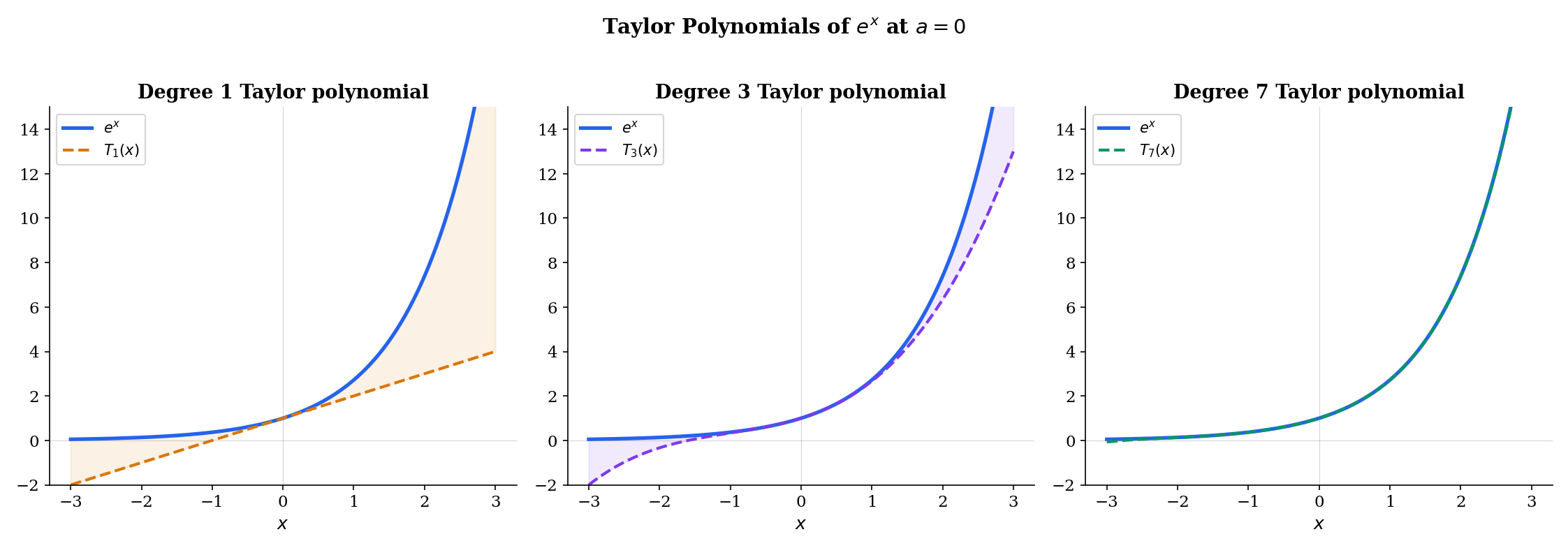
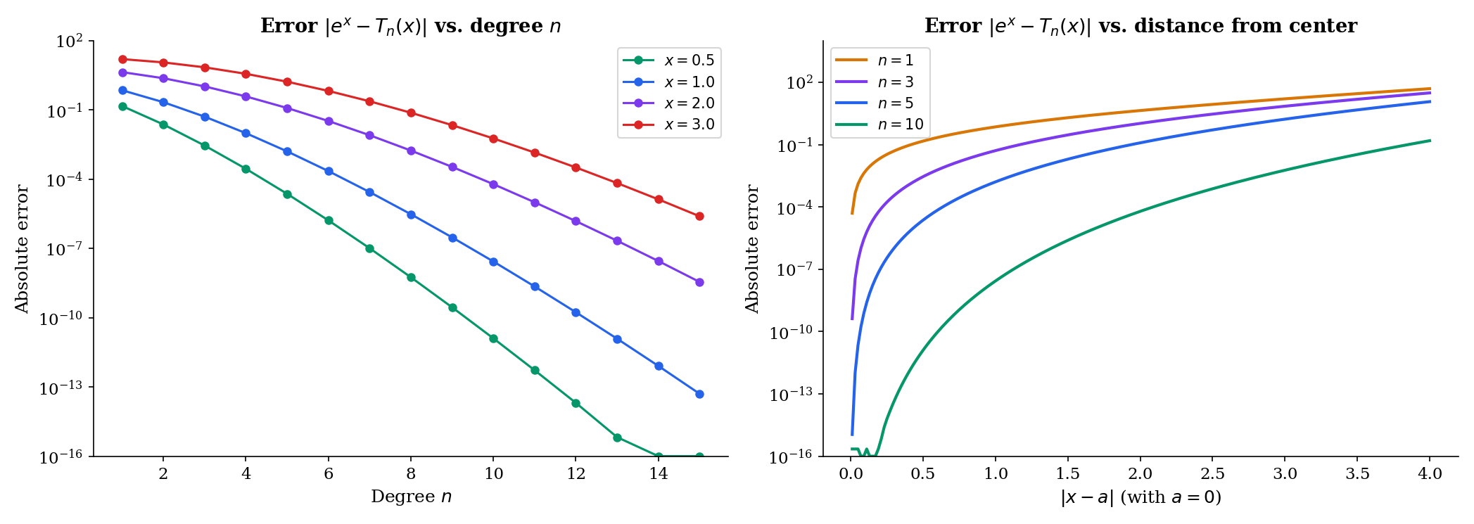
📝 Example 4 (Taylor polynomials of eˣ at a = 0)
Since all derivatives of equal , we have for all :
As increases, approximates over a wider and wider interval. Try increasing the degree in the explorer below to watch the polynomial “hug” the exponential.
📝 Example 5 (Taylor polynomials of sin(x) at a = 0)
The derivatives of cycle: At : , , , , ,
Only odd terms survive:
The pattern reflects the odd symmetry of — an odd function’s Taylor series has only odd powers.
Taylor’s Theorem (with Remainder)
The Taylor polynomial approximates — but how well? Taylor’s theorem gives a quantitative error bound via the remainder term .
🔷 Theorem 5 (Taylor's Theorem (Lagrange Remainder))
Let be -times differentiable on an open interval containing and . Then
for some between and .
Proof.
We prove this by applying Rolle’s theorem to a carefully constructed auxiliary function. Fix and define
where is the degree- Taylor polynomial of centered at (evaluated at the variable ), and is a constant chosen so that .
First note that , so .
Next, the condition gives
Our goal is to show that for some between and .
Since , Rolle’s theorem gives some between and with . We differentiate a total of times. At each stage, the polynomial terms from lose one degree, and after differentiations the Taylor polynomial terms vanish entirely:
(since differentiates times to , and is a degree- polynomial whose -th derivative is ).
By applying Rolle’s theorem successively — gives a zero of , which combined with gives a zero of , and so on — we obtain a point between and with . Setting this to zero:
Combining with the expression gives the Lagrange remainder:
Note: The base case gives , which is exactly the Mean Value Theorem. Taylor’s theorem is the higher-order generalization of the MVT.
💡 Remark 4 (The integral form of the remainder)
An alternative expression for the remainder is
This avoids the unknown point and is sometimes more useful for estimation. The integral form is proved using integration by parts in The Riemann Integral & FTC, §9.
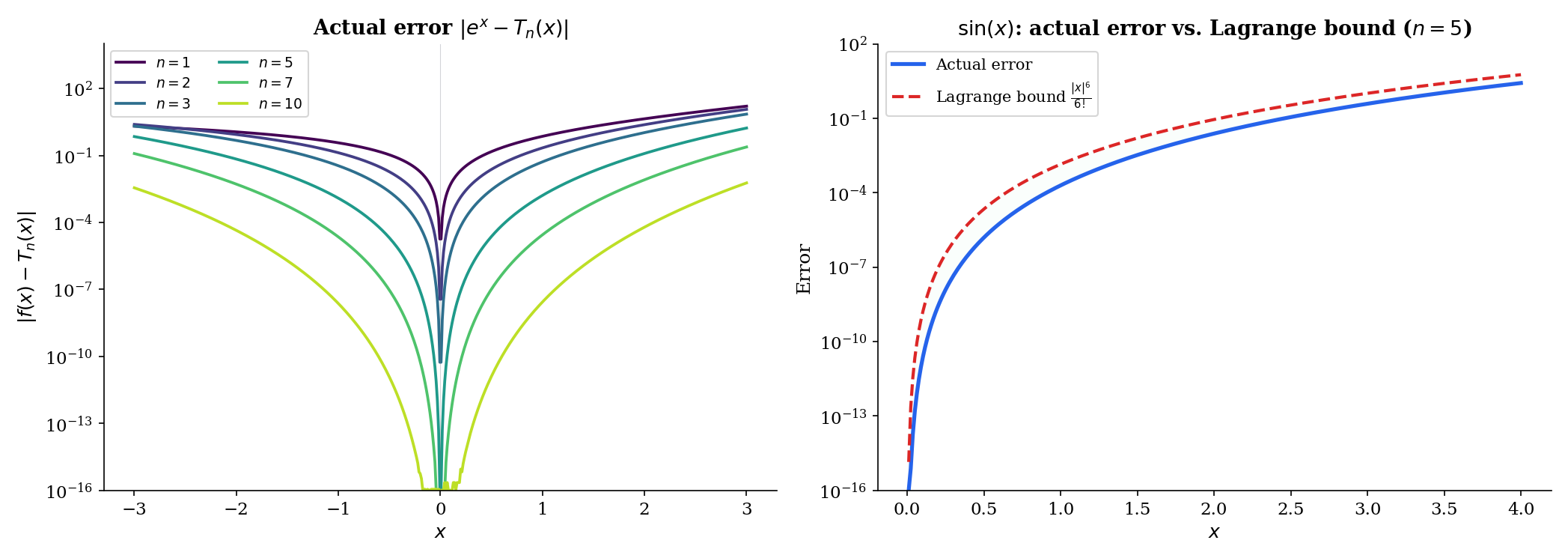
📝 Example 6 (Taylor remainder for eˣ)
For with : all derivatives are , so for some between and . The Lagrange remainder is
For any fixed , as because the factorial grows faster than any power . This proves that converges for all .
📝 Example 7 (Taylor remainder for sin(x))
For with : all derivatives of are bounded by in absolute value, so
for any fixed . The Maclaurin series of converges to for all .
When Taylor Series Fail
Not every smooth function equals its Taylor series. The fact that Taylor polynomials approximate well locally (small , fixed ) does not guarantee that the Taylor series converges to (fixed , ).
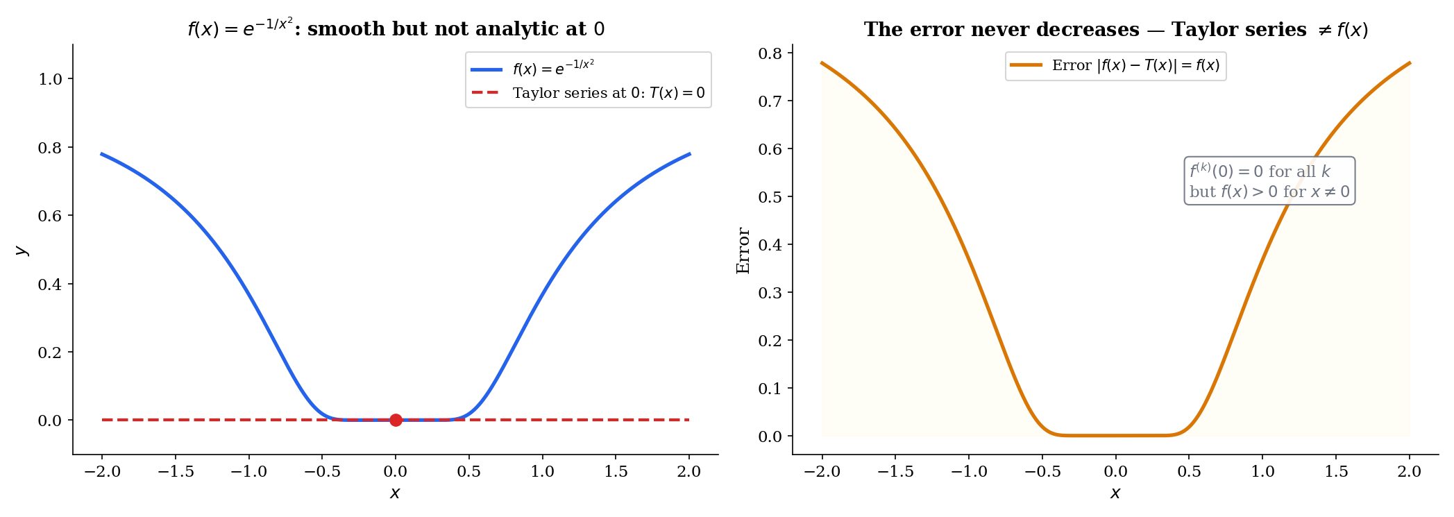
📝 Example 8 (Smooth but not analytic: f(x) = e^{−1/x²})
Define
This function is (infinitely differentiable) everywhere. At , one can show by induction (using L’Hôpital’s Rule from §5 at each step) that for all . So the Taylor series at is
but for all . The Taylor series converges (to ), but it does not converge to . The function “flattens” against zero so aggressively at that no polynomial can detect the non-zero values away from the origin.
📐 Definition 2 (Analytic Function)
A function is analytic at if its Taylor series at converges to in some neighborhood of : there exists such that for all .
Most functions encountered in practice — , , , polynomials, rational functions away from poles — are analytic. The function is the standard example of smooth but not analytic.
💡 Remark 5 (Smooth vs. analytic in ML)
In practice, loss functions in ML are typically compositions of analytic functions (exponentials, logarithms, polynomials), so the Taylor expansion is a reliable local model. ReLU is piecewise linear (hence piecewise analytic). The distinction between smooth and analytic matters more in theory — the existence of smooth bump functions (which are with compact support and are not analytic) is essential for partition-of-unity arguments in differential geometry. (→ formalML: Smooth Manifolds)
Connections to Statistics
Taylor expansion is the analytical engine behind almost every asymptotic result in statistics. The CLT, the asymptotic normality of the MLE, Laplace approximation, the delta method — all are second-order Taylor stories with carefully controlled remainders.
The CLT via characteristic functions
The characteristic-function proof of the Central Limit Theorem expands to second order in near : . Summing independent terms and rescaling gives the Gaussian characteristic function in the limit. The Mean Value Theorem controls the remainder. See formalStatistics Central Limit Theorem.
Laplace approximation and BIC
Laplace approximation expands the log-posterior to second order around the MAP : The Bayesian Information Criterion is the asymptotic form of this expansion. See formalStatistics Bayesian Model Comparison & BMA.
Asymptotic normality of the MLE
follows from a Taylor expansion of the score: . Solving for and rescaling produces the limit distribution. See formalStatistics Maximum Likelihood.
Cumulants from the cumulant generating function
The cumulant generating function has Taylor coefficients equal to the cumulants : . The exponential-family structure makes these derivatives tractable in closed form; the cumulants are the natural moments of choice for both inference and asymptotic expansions. See formalStatistics Exponential Families.
Connections to ML — Taylor Expansion in Optimization
Taylor expansion is not just used in ML proofs — it is the primary analytical technique for understanding optimization algorithms.
The descent lemma
Suppose is twice differentiable and is -Lipschitz: . By the second-order Taylor expansion with Lagrange remainder (in one dimension, this is Theorem 5 with ):
for some between and . Since (the Lipschitz gradient condition — Corollary 3 applied to ), we get the descent lemma:
Setting (a gradient descent step with learning rate ) and simplifying:
Each GD step decreases by at least . This is the foundation of every gradient descent convergence proof.
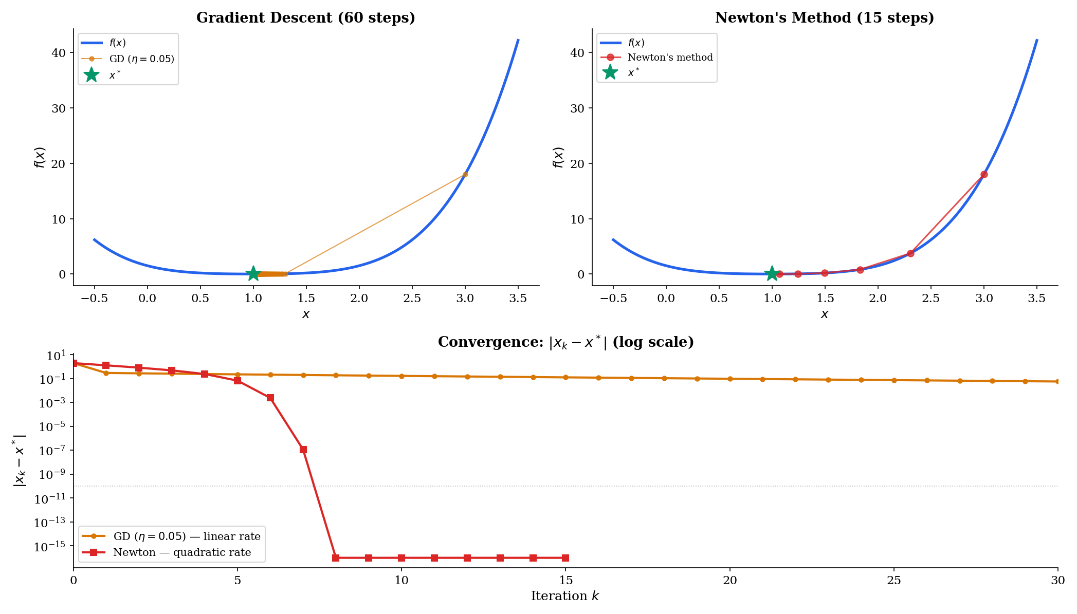
Newton’s method
Newton’s method approximates by its local quadratic Taylor model:
Minimizing gives , yielding the Newton update:
For root-finding (solve ), the linear Taylor model gives . Near a root, the Taylor remainder analysis shows the error satisfies — quadratic convergence. Each iteration roughly doubles the number of correct digits.
Convergence rate comparison
Using Taylor expansion, we can compare:
- Gradient descent (first-order, uses model): linear convergence for some .
- Newton’s method (second-order, uses model): quadratic convergence , which is doubly exponential decay.
The practical trade-off: Newton needs (the Hessian in higher dimensions), which is expensive to compute. This is why quasi-Newton methods like L-BFGS exist — they approximate the second-order Taylor model cheaply. (→ formalML: Gradient Descent)
Computational Notes
Taylor approximation is straightforward to implement numerically. In Python:
import numpy as np
from math import factorial

def taylor_polynomial(f_derivs, a, n, x):
    """Evaluate the degree-n Taylor polynomial of f at x.
    f_derivs: list of derivative functions [f, f', f'', ...]
    """
    return sum(f_derivs[k](a) / factorial(k) * (x - a)**k for k in range(n + 1))

# Taylor polynomials of e^x at a = 0
x = np.linspace(-3, 3, 1000)
for n in [1, 3, 5, 10]:
    T_n = sum((x**k) / factorial(k) for k in range(n + 1))
    max_error = np.max(np.abs(np.exp(x) - T_n))
    print(f"T_{n}: max error on [-3,3] = {max_error:.6e}")
For Newton’s method in practice, SciPy provides scipy.optimize.minimize(f, x0, method='Newton-CG'), which implements a Newton-conjugate gradient method that approximates the Hessian-vector product without forming the full Hessian matrix.
Connections & Further Reading
Prerequisites — topics you need first
The Derivative & Chain Rule
The derivative definition and differentiation rules from Topic 5 are the raw material. Rolle's theorem and MVT are statements about the derivative — they assert the existence of points where f' takes specific values. Taylor's theorem builds polynomial approximations from higher-order derivatives f', f'', ..., f⁽ⁿ⁾.
Completeness & Compactness
Rolle's theorem requires the Extreme Value Theorem: a continuous function on [a,b] achieves its maximum and minimum. The EVT was proved in Topic 3 using compactness (Heine-Borel). The chain Rolle → MVT → Taylor is built on the compactness foundation.
Sequences, Limits & Convergence
Taylor remainder estimation involves limits of the form Rₙ(x) → 0 as n → ∞. Convergence rate analysis (linear, quadratic) for Newton's method uses the sequence convergence framework from Topic 1.
Epsilon-Delta & Continuity
The continuity and differentiability hypotheses in Rolle's theorem and MVT are formalized using the ε-δ framework from Topic 2. L'Hôpital's Rule requires careful handling of limits of ratios.
Where this leads — next in formalCalculus
On to formalStatistics — where this calculus powers inference
Kernel Density Estimation
Topic 30's KDE bias derivation (§30.4) Taylor-expands the unknown density $f$ around $x$ to second order; §30.6's bandwidth optimization Taylor-expands AMISE around $h^\ast$. Both invoke the second-order Taylor theorem with Lagrange/Peano remainder developed here.
Central Limit Theorem
The characteristic-function proof of the CLT expands log φ_X(t) to second order in t near 0: log φ_X(t) = iμt - σ²t²/2 + o(t²). Summing and rescaling gives the Gaussian characteristic function in the limit — pure Taylor expansion plus an MVT-controlled remainder.
Bayesian Model Comparison And Bma
Laplace approximation approximates ∫ exp(ℓ(θ)) dθ ≈ exp(ℓ(θ̂)) · (2π)^(d/2) / √det(-∇²ℓ(θ̂)) — a 2nd-order Taylor expansion of the log-posterior around the MAP. The BIC penalty falls out of this expansion.
Maximum Likelihood
Asymptotic normality of the MLE √n(θ̂ - θ_0) ⟹ N(0, I⁻¹) follows from a Taylor expansion of the score: 0 = U_n(θ̂) ≈ U_n(θ_0) + H_n(θ_0)(θ̂ - θ_0), solved for (θ̂ - θ_0) and rescaled.
Exponential Families
The cumulant generating function K(t) = log M_X(t) has Taylor coefficients equal to the cumulants κ_n: K(t) = Σ κ_n t^n/n!. The exponential-family structure makes these derivatives tractable in closed form.
On to formalML — where this calculus powers ML
Gradient Descent
The descent lemma — the cornerstone inequality in gradient descent convergence proofs — is a direct consequence of second-order Taylor expansion with Lipschitz gradient. Newton's method replaces f with its local quadratic Taylor model at each step, achieving quadratic convergence where GD achieves only linear.
Proximal Methods
Proximal operators minimize f(y) + (1/2t)‖y - x‖², which is the second-order Taylor model of f at x plus a quadratic penalty. The Moreau envelope uses the same Taylor-inspired local quadratic structure.
Smooth Manifolds
Taylor expansion on manifolds generalizes via the exponential map. The MVT extends to curves on manifolds, and Taylor approximation in local coordinates is the foundation for Riemannian optimization.
Causal Inference Methods
The §6.3 product-of-errors decomposition of the AIPW score and the §8.2 Neyman-orthogonality derivation use Taylor expansion of the score around the true nuisances; the mean-value-theorem argument that bias has a second-order remainder in the nuisance estimation error is what licenses ML nuisances in the DML framework.
Kernel Regression
The §3.2 second-order Taylor expansion of $f_X(x + hu)$ and $g(x + hu) = m(x + hu)\,f_X(x + hu)$ around $x$, with explicit $h^2$ remainder term, is the load-bearing technical move of the entire bias derivation. The §6.3 multivariate version uses the Hessian $\nabla^2 m$ in place of the second derivative.
Local Regression
Taylor expansion to order $p+1$ is the load-bearing move of the §4 bias derivation at general degree $p$ — higher-order than the order-2 expansion used in Nadaraya–Watson kernel regression. The §4.1 residual-decomposition argument absorbs the first $p+1$ Taylor terms via column-space projection, leaving only the $(p+1)$-st derivative remainder to drive the bias.
Semiparametric Inference
§3.1's von Mises expansion is the functional version of Taylor's theorem in a Hilbert space. §5.3's one-step asymptotic-normality theorem and §7.2's product-of-errors $R_2$ derivation both reduce to careful first- and second-order Taylor analyses of the functional $\psi$ at the truth.
Structural Risk Minimization
Polynomial-Taylor expansion intuition for the bias of $\mathcal{H}_k$ on smooth targets: the $k = 3$ class captures the leading Taylor terms of $\sin(\pi x) \approx \pi x - (\pi x)^3/6$, which is why bias drops sharply at $k = 3$ in the §1.5 Monte Carlo. Taylor-remainder bounds control $L^*(\mathcal{H}_k)$ as a function of target smoothness.
Variational Bayes For Model Selection
§3's Laplace approximation is a second-order Taylor expansion of $\log p(x, \theta)$ around the MAP, with the remainder term controlling asymptotic accuracy. Tierney–Kadane's (1986) refined Laplace approximation uses higher-order Taylor terms for marginal-density accuracy beyond the leading-order Schwarz form.
References
- book Abbott (2015). Understanding Analysis Chapter 5 develops MVT from Rolle's theorem with exceptional clarity; Chapter 6 covers Taylor's theorem — the primary reference for our rigorous-but-accessible approach
- book Rudin (1976). Principles of Mathematical Analysis Chapter 5 on differentiation covers MVT and Taylor's theorem in the definitive compact style
- book Spivak (2008). Calculus Chapters 11–12 develop MVT and Taylor's theorem with unmatched geometric intuition alongside full rigor — exceptional treatment of the Taylor remainder
- book Boyd & Vandenberghe (2004). Convex Optimization Section 9.1 on unconstrained minimization — the descent lemma and convergence rate proofs that directly use Taylor expansion
- book Nesterov (2004). Introductory Lectures on Convex Optimization Chapter 1 develops the Lipschitz gradient framework and descent lemma — the canonical application of Taylor expansion to optimization convergence analysis