Calculus of Variations
Optimizing functionals — the Euler-Lagrange equation, Sobolev spaces, and the direct method
Abstract. The calculus of variations extends optimization from finite-dimensional spaces to spaces of functions. Given a functional — a map from a function space to the reals — we ask: which function minimizes it? The Euler-Lagrange equation provides the necessary condition, the second variation tests sufficiency, and the direct method of the calculus of variations proves existence. Sobolev spaces supply the natural domain, and the Lax-Milgram theorem connects variational problems to weak solutions of PDEs. These ideas underpin physics-informed neural networks, optimal transport, variational autoencoders, and diffusion models.
1. Overview and Motivation
In a physics-informed neural network, the loss function is a functional — it maps a function (the neural network) to a real number (the PDE residual). Minimizing it is not ordinary optimization over parameters; it is optimization over a function space. The loss is literally
where is a differential operator and is the network output viewed as a function. This is the calculus of variations in its modern incarnation.
The arc of Track 8 has been a staircase of abstraction, each step adding one axiom and gaining strictly stronger conclusions:
- Metric spaces (Topic 29): distances → completeness → fixed-point theorems.
- Normed/Banach spaces (Topic 30): length → bounded operators → the big four theorems.
- Inner product/Hilbert spaces (Topic 31): angles → orthogonality → projection, Riesz representation, spectral decomposition.
- Calculus of variations (this topic): perturbation → optimization over function spaces → Euler-Lagrange equations, direct method, eigenvalue problems.
The key idea of finite-dimensional optimization is: which point minimizes ? Set the derivative to zero and solve. The calculus of variations asks a harder question: which function minimizes ? The answer requires a new derivative (the first variation, a directional derivative in function space), a new existence theory (the direct method, using weak compactness in Hilbert spaces), and a new domain (the Sobolev spaces that are the natural home for variational problems).
This is the final topic in formalCalculus — the capstone of both Track 8 and the entire 32-topic journey from epsilon-delta definitions to functional analysis. Let’s begin.
2. Functionals and Their Domains
📐 Definition 1 (Functional)
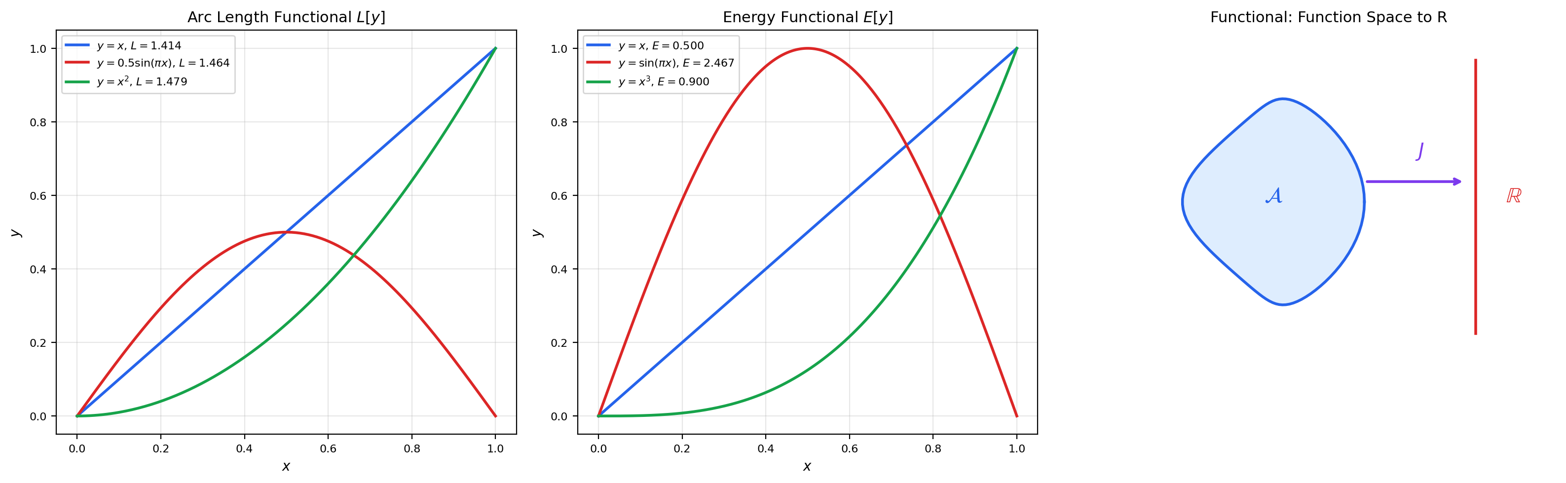
A functional is a map , where is a subset of a function space. We write rather than to distinguish functionals (which eat functions) from ordinary functions (which eat numbers).
📝 Example 1 (Arc Length Functional)
The arc length of a curve is
This maps each function to a non-negative real number.
📝 Example 2 (Energy Functional)
The Dirichlet energy
measures the total “kinetic energy” stored in the gradient of . Minimizing subject to boundary conditions , yields the straight line .
📝 Example 3 (Action Functional (Lagrangian Mechanics))
In classical mechanics, the action is
where is the Lagrangian (kinetic minus potential energy). Hamilton’s principle: the physical trajectory extremizes the action.
📝 Example 4 (ML Loss as a Functional)
A PINN loss is a functional on the space of neural network functions:
The parameters parameterize a submanifold of function space; optimization over is a finite-dimensional proxy for the infinite-dimensional variational problem.
💡 Remark 1 (Hilbert-Space Vocabulary Refresh)
We will use the inner-product and Hilbert-space machinery from Topic 31 throughout this topic. Recall: a Hilbert space is a complete inner-product space. The projection theorem guarantees a unique closest point in any closed convex subset. The Riesz representation theorem identifies the dual space with itself. These are not just background — they are the active ingredients in the direct method (Section 8) and the Lax-Milgram theorem (Section 9).
3. The First Variation
The first variation is the directional derivative of a functional — the rate of change of when we perturb in the direction .
📐 Definition 2 (First Variation (Gâteaux Derivative))
The first variation of at in the direction is
provided the limit exists for all admissible perturbations (typically , meaning smooth functions vanishing at the boundary). If for all , we call a critical point (or extremal) of .
This is the function-space analogue of the gradient. In , a critical point of satisfies . In function space, a critical point of satisfies for all directions . The Euler-Lagrange equation (next section) is what looks like when has the integral form .
🔷 Theorem 1 (Fundamental Lemma of the Calculus of Variations)
If and
then for all .
Proof. Suppose for contradiction that at some . Without loss of generality, assume . By continuity of , there exists such that for all .
Choose to be a smooth bump function supported on with and . For instance, take
Then , and
This contradicts for all . Therefore .
📝 Example 5 (First Variation of the Energy Functional)
For :
Integrating by parts (with ): . Setting this to zero for all and applying the fundamental lemma gives — the extremal is a straight line.
📝 Example 6 (First Variation of the Arc Length Functional)
For , a similar computation gives
After integration by parts, the Euler-Lagrange equation is , which implies is constant — again, a straight line (which minimizes arc length between two points in the plane).
💡 Remark 2 (Connection to Taylor Expansion)
The first variation is a Taylor expansion in function space. Writing as a power series in (cf. Topic 6):
The first variation is the linear term; the second variation (Section 6) is the quadratic term. A critical point has ; a minimum requires .

4. The Euler-Lagrange Equation
This is the central result of the classical calculus of variations: a necessary condition for a curve to be an extremal of a functional.
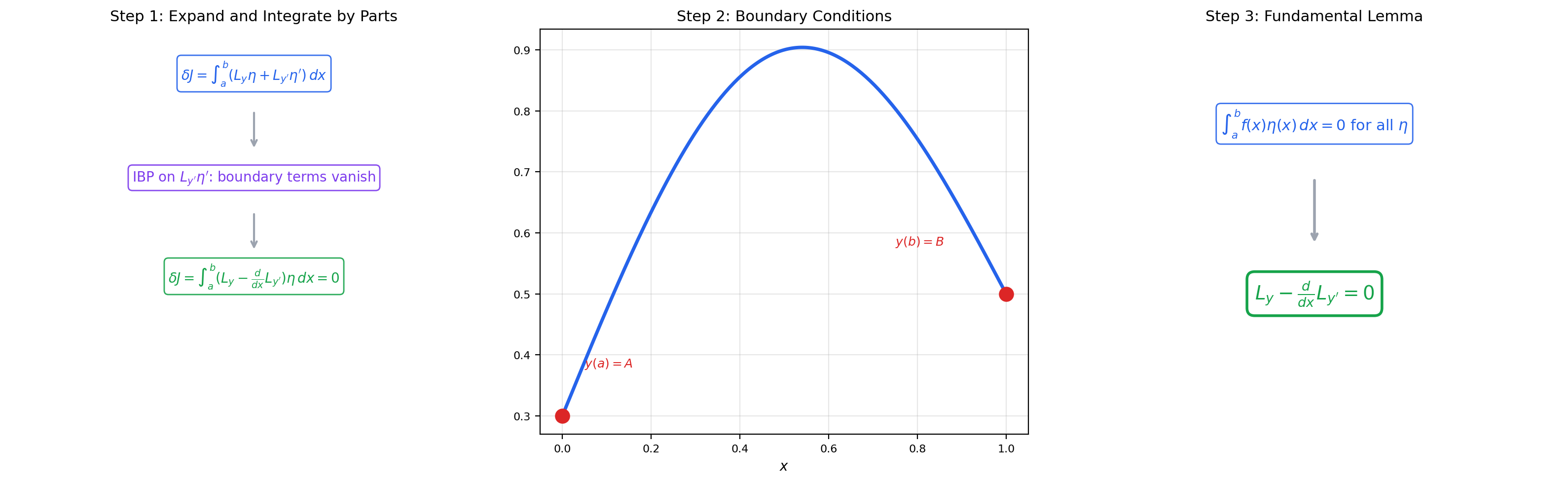
🔷 Theorem 2 (The Euler-Lagrange Equation)
Let be in all arguments, and let . If is an extremal of (i.e., for all ), then satisfies the Euler-Lagrange equation:
Proof. We proceed in six steps.
Step 1: Expand the perturbed functional. Replace by in :
Step 2: Differentiate under the integral. By the chain rule:
Step 3: Integrate the second term by parts. Writing and , we get and :
Step 4: Apply the boundary conditions. Since , the boundary term vanishes:
Step 5: Combine and factor. Substituting back:
for all .
Step 6: Apply the fundamental lemma. By Theorem 1, since the expression in brackets is continuous and its integral against every smooth compactly-supported vanishes, we conclude
on .
The explorer above lets you drag control points on a candidate curve and watch the functional value update in real time. The green curve is the analytic Euler-Lagrange solution — it achieves the minimum. The vs plot on the right confirms that the functional value has a minimum at when the candidate is the E-L solution.
📝 Example 7 (Shortest Path (Straight Line))
For : and . The Euler-Lagrange equation gives , so . The extremal is a straight line — as expected.
📝 Example 8 (Harmonic Oscillator from Variational Principle)
The action has Lagrangian . The Euler-Lagrange equation yields — Newton’s second law for a spring.
💡 Remark 3 (Natural vs. Essential Boundary Conditions)
The proof of the Euler-Lagrange equation assumed (Dirichlet/essential boundary conditions). If we allow , the boundary term must vanish independently, giving the natural boundary condition . This is important in finite element methods.
5. Classical Examples
These are the problems that launched the calculus of variations in the 17th and 18th centuries.
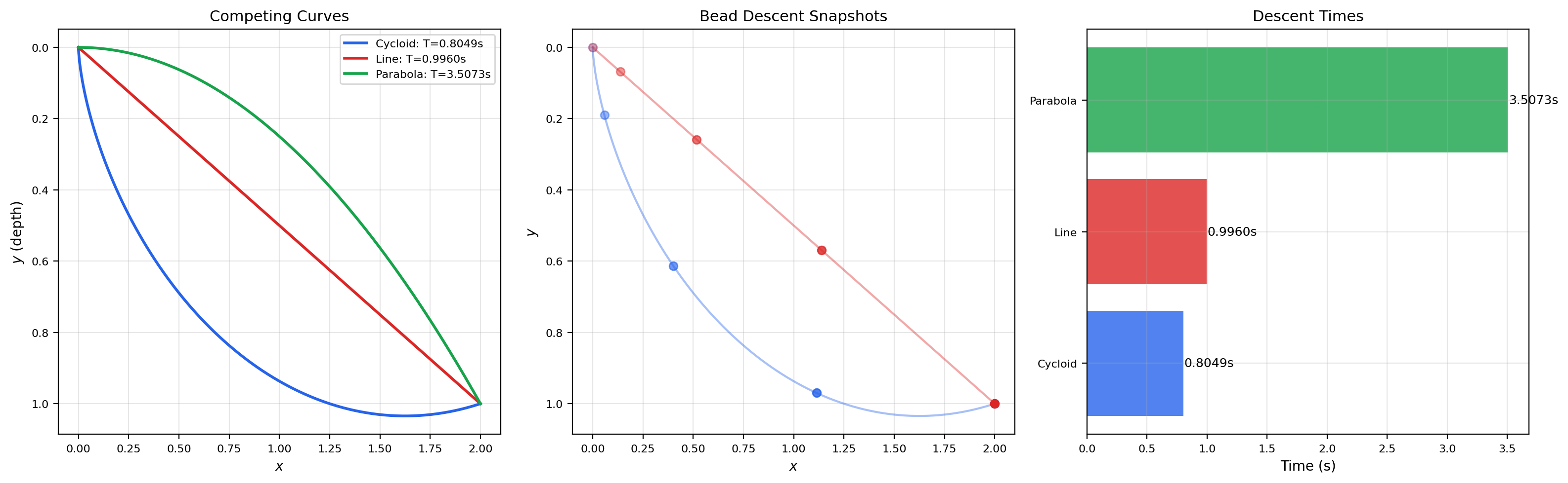
📝 Example 9 (The Brachistochrone Problem)
Problem: Find the curve of fastest descent under gravity from point to point , starting from rest.
The descent time is . The Euler-Lagrange equation (with Lagrangian ) yields . The solution is a cycloid:
where is determined by the endpoint condition. The cycloid is about 19% faster than the straight-line path.
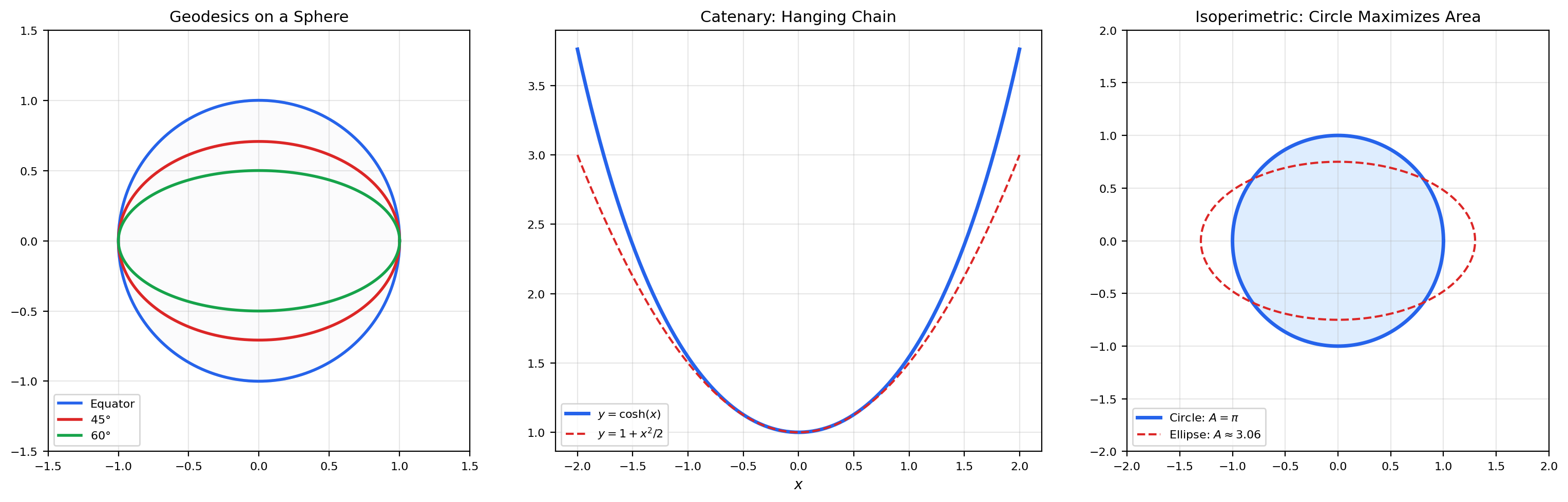
📝 Example 10 (Geodesics on Surfaces)
A geodesic minimizes the arc-length functional (cf. Topic 20). On a sphere of radius , the Euler-Lagrange equation yields great circles — the shortest paths between points on the sphere.
📝 Example 11 (The Catenary)
A flexible chain of uniform density hanging under gravity adopts the shape that minimizes potential energy subject to the constraint of fixed length. The Euler-Lagrange equation with a Lagrange multiplier gives the catenary:
where depends on the chain length and endpoint separation.
📝 Example 12 (The Isoperimetric Problem)
Problem: Among all closed curves of fixed perimeter , which one encloses the maximum area?
This is a constrained variational problem. We maximize subject to . Using a Lagrange multiplier , the Euler-Lagrange equation for yields a circle of radius .
💡 Remark 4 (Constrained Variations and Lagrange Multipliers)
Constrained variational problems (like the isoperimetric problem) add a side condition to the functional . The method of Lagrange multipliers in function space: extremize over all and . This is the infinite-dimensional prototype for Lagrangian duality in optimization.
6. The Second Variation and Sufficient Conditions
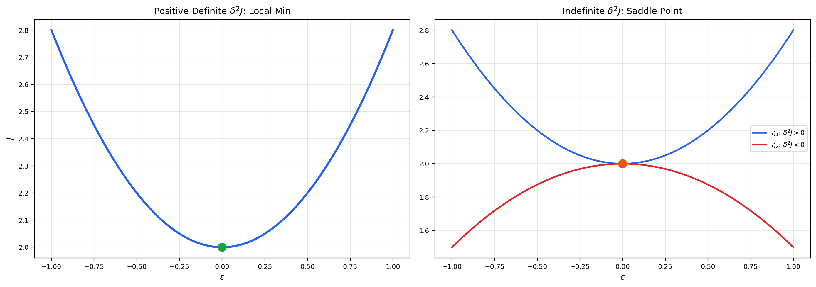
The Euler-Lagrange equation is a necessary condition — it finds critical points. But is a critical point a minimum, a maximum, or a saddle point? The second variation answers this question, just as the second derivative does in single-variable calculus.
📐 Definition 3 (Second Variation)
The second variation of at an extremal in the direction is
For , this becomes
🔷 Theorem 3 (Legendre's Necessary Condition)
If is a local minimizer of , then
Proof. If is a minimizer, then for all admissible . Take to be a tall, narrow bump centered at . In the limit, the term dominates, and we need . Formally: choose where is a standard mollifier. Then , and
For as , we need .
📐 Definition 4 (Conjugate Points and the Jacobi Equation)
A point is conjugate to along the extremal if there exists a non-trivial solution of the Jacobi equation
satisfying . Conjugate points are where nearby extremals refocus.
🔷 Theorem 4 (Jacobi's Sufficient Condition)
If is an extremal of with on (strengthened Legendre), and there are no conjugate points in , then is a (strict) local minimum.
Proof outline. The absence of conjugate points ensures that the Jacobi equation has no non-trivial solutions vanishing at both endpoints. This means the quadratic form is positive definite on the space of admissible variations, which implies is a local minimum. The full proof uses the theory of fields of extremals.
📝 Example 13 (Second Variation of the Energy Functional)
For : , , . So , with equality only if , i.e., (since ). The Jacobi equation is with , giving . This has no zero in , so there are no conjugate points. The straight line is a strict minimum.
💡 Remark 5 (The Second Variation as a Function-Space Hessian)
The second variation is the function-space analogue of the Hessian matrix. In , a critical point is a minimum if the Hessian is positive definite. In function space, a critical point is a minimum if is positive definite on the space of admissible perturbations. This connects the calculus of variations to the spectral theory of differential operators — the Jacobi equation defines a self-adjoint operator whose eigenvalues determine whether is positive definite. This closes the obligation planted in Topic 29 about the variational characterization of extrema in infinite dimensions.
7. Sobolev Spaces
Classical solutions (smooth functions satisfying the Euler-Lagrange equation pointwise) do not always exist. The natural function spaces for variational problems are Sobolev spaces — spaces of functions with weak derivatives in .
📐 Definition 5 (Weak Derivative)
A function has a weak derivative if
This is the integration-by-parts formula with no boundary term (since vanishes at the boundary). The weak derivative agrees with the classical derivative when is classically differentiable, but extends to a much larger class of functions.
📐 Definition 6 (Sobolev Space H¹(Ω) and H¹₀(Ω))
The Sobolev space consists of all functions with weak derivatives in :
equipped with the inner product .
The subspace consists of functions that vanish on the boundary (in the trace sense). This is the natural space for Dirichlet boundary conditions.
🔷 Theorem 5 (H¹₀(Ω) Is a Hilbert Space)
with the inner product is a Hilbert space (a complete inner product space).
Proof. We need to show completeness. Let be a Cauchy sequence in . Then and are both Cauchy in . Since is complete, there exist with and in . We verify is the weak derivative of : for any ,
so in the weak sense. Hence . Since , the boundary values (traces) converge to zero, so . Thus in .
🔷 Theorem 6 (Poincaré Inequality)
For bounded , there exists such that
Proof (for ). By the fundamental theorem of calculus and Cauchy-Schwarz:
Integrating over : . So .
The Poincaré inequality says that on , the seminorm is equivalent to the full norm. This is crucial for the coercivity arguments in the direct method.
🔷 Theorem 7 (Rellich-Kondrachov Compactness Theorem)
For bounded with Lipschitz boundary, the embedding is compact: every bounded sequence in has a subsequence converging in .
Proof deferred. The full proof requires approximation theory and the Arzelà-Ascoli theorem (cf. Topic 29). We state this result because it is essential for the direct method: it converts weak convergence in to strong convergence in .
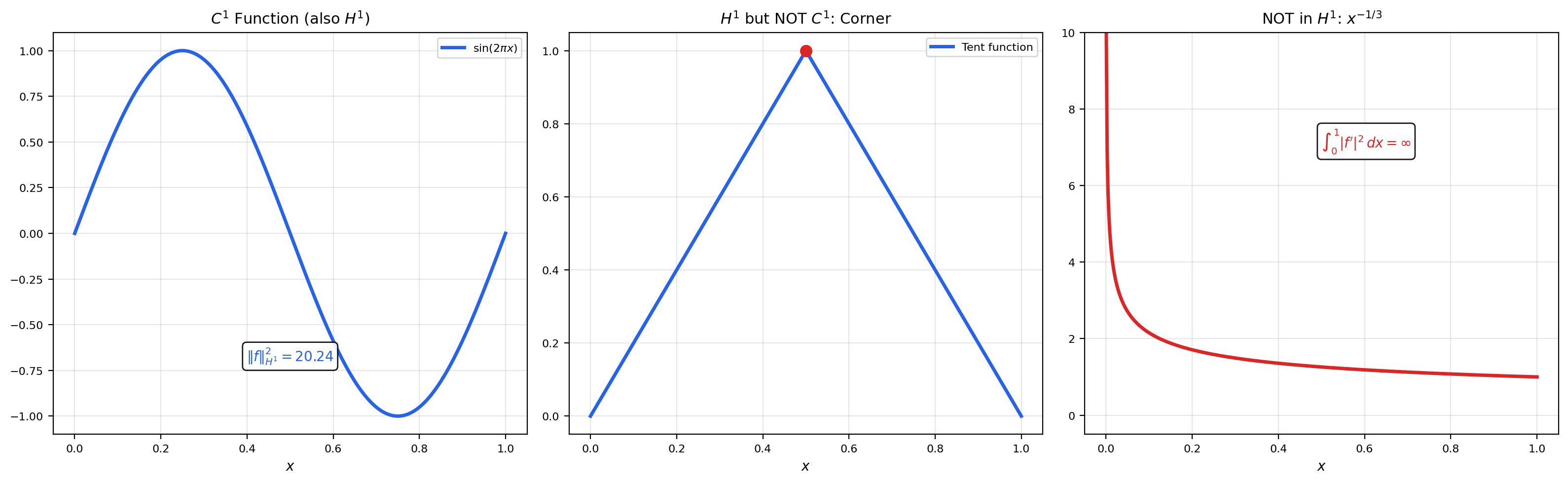
📝 Example 14 (Functions in H¹ That Are Not in C¹)
The tent function on has a corner at and is not classically differentiable there. But it has a weak derivative: on and on . Since both and are in , we have . Its squared norm is , so .
In contrast, on has , and . So .
💡 Remark 6 (Sobolev Spaces as Hilbert Spaces)
The key point: with the inner product is a Hilbert space (Theorem 5). This means we can apply the entire Hilbert-space toolkit from Topic 31 — projection theorem, Riesz representation, spectral theory — to variational problems posed on Sobolev spaces. This closes the obligation from Topic 31 and Topic 23 to explain why Sobolev spaces are the right function spaces for PDEs.
8. The Direct Method
The direct method is the crown jewel of the modern calculus of variations. It answers the existence question: does a minimizer exist? Where the Euler-Lagrange equation finds candidates, the direct method proves that a minimizer is actually achieved.
📐 Definition 7 (Coercivity and Weak Lower Semicontinuity)
A functional on a Hilbert space is:
- Coercive if as .
- Weakly lower semicontinuous (w.l.s.c.) if (weak convergence) implies .
🔷 Theorem 8 (The Direct Method of the Calculus of Variations)
Let be a reflexive Banach space (e.g., a Hilbert space) and be coercive and weakly lower semicontinuous. Then attains its infimum: there exists with .
Proof. We proceed in four steps.
Step 1: Bounded minimizing sequence. Let and choose a minimizing sequence with . By coercivity, is bounded: if , then , contradicting .
Step 2: Weak compactness. Since is reflexive and is bounded, by the Eberlein-Šmulian theorem (the sequential version of the Banach-Alaoglu theorem for reflexive spaces), there exists a subsequence and with (weak convergence).
Step 3: Lower semicontinuity. Since is weakly lower semicontinuous:
Step 4: Conclusion. By definition, . Combined with Step 3, . The infimum is attained.
The explorer shows the direct method in action: a minimizing sequence converges to the minimizer , with descending to .
📝 Example 15 (Existence of Minimizer for the Dirichlet Energy)
The Dirichlet energy on satisfies:
- Coercivity: By Poincaré, .
- Weak lower semicontinuity: The norm is w.l.s.c., and (using the equivalent norm from Poincaré).
By the direct method, a minimizer exists. This is the variational proof of existence for the Poisson equation with Dirichlet boundary conditions.
📝 Example 16 (Best Approximation as a Variational Problem)
💡 Remark 7 (The Direct Method as the Infinite-Dimensional Extreme Value Theorem)
In finite dimensions, the extreme value theorem says: a continuous function on a compact set attains its extrema. The direct method is the infinite-dimensional version. Coercivity provides the “compact set” (bounded sublevel sets), weak lower semicontinuity provides “continuity” (in the weak topology), and reflexivity provides “compactness” (Eberlein-Šmulian). This closes the staircase from the Bolzano-Weierstrass theorem in Topic 29 to the direct method here.
![Minimizing sequence converging: curves y_n, functional values J[y_n] descending, weak limit as minimizer.](/images/topics/calculus-of-variations/direct-method.png)
9. Weak Solutions and the Lax-Milgram Theorem
The Lax-Milgram theorem is the bridge between variational problems and PDEs: it converts a variational problem into a well-posed operator equation.
📐 Definition 8 (Weak Solution of a PDE)
A function is a weak solution of the boundary value problem (with ) if
This is obtained by multiplying the PDE by a test function , integrating by parts, and dropping the boundary term (since ).
📐 Definition 9 (Bilinear Form — Coercivity and Boundedness)
A bilinear form on a Hilbert space is:
- Bounded (continuous) if for some .
- Coercive if for some .
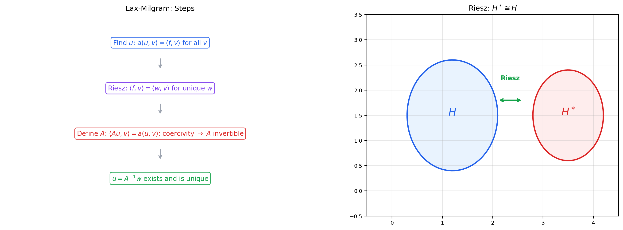
🔷 Theorem 9 (Lax-Milgram Theorem)
Let be a Hilbert space, a bounded, coercive bilinear form, and a bounded linear functional. Then there exists a unique such that
Proof. The key is to use the Riesz representation theorem from Topic 31.
Step 1: Define the operator . For each fixed , the map is a bounded linear functional on . By the Riesz representation theorem, there exists a unique such that for all . The map is linear and bounded with .
Step 2: Show is bijective. Coercivity gives , so:
This means is injective and has closed range.
Step 3: Show the range is dense. If , then , but coercivity gives , so . Hence , meaning is dense in .
Step 4: Conclude. Since is both closed and dense, is surjective. Hence is bijective with bounded inverse ().
Now apply Riesz again: corresponds to some with . Set . Then for all .
📝 Example 17 (Weak Solution of Poisson's Equation)
For on with : take , , . By Poincaré, is coercive: . By Cauchy-Schwarz, is bounded. Lax-Milgram gives the unique weak solution .
📝 Example 18 (Weak Solution of the Sturm-Liouville Problem)
For on with : take . If and , then is coercive and bounded. Lax-Milgram applies.
💡 Remark 8 (From Lax-Milgram to Finite Elements)
The finite element method discretizes the Lax-Milgram problem: replace by a finite-dimensional subspace (e.g., piecewise-linear functions on a mesh), and solve for all . This is a finite linear system where is the stiffness matrix. The Lax-Milgram theorem guarantees that the stiffness matrix is invertible (because is coercive on too).
10. Eigenvalue Problems and the Rayleigh Quotient
The variational characterization of eigenvalues connects the spectral theory from Topic 31 to the calculus of variations.
📐 Definition 10 (Sturm-Liouville Eigenvalue Problem)
The Sturm-Liouville eigenvalue problem is: find non-trivial and such that
The eigenvalues are () with eigenfunctions .
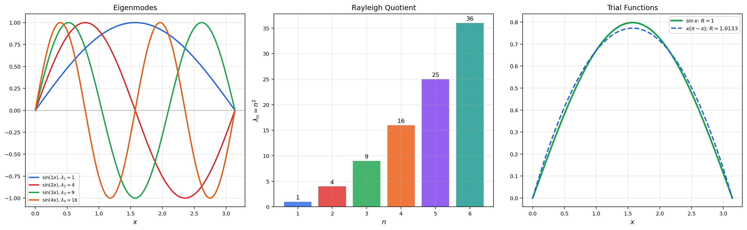
🔷 Theorem 10 (Variational Characterization of the First Eigenvalue)
The first eigenvalue of on with Dirichlet conditions is
is the Rayleigh quotient. The minimum is achieved by with .
Proof. We use the weak formulation. Multiply by and integrate by parts:
Setting : , so for any eigenfunction.
Now we show is the minimum of . Expand in the eigenfunction basis: . By Parseval’s identity:
Therefore , with equality when for , i.e., .
🔷 Theorem 11 (Min-Max Principle (Courant-Fischer))
The -th eigenvalue is
Proof outline. This follows from the spectral theorem for compact self-adjoint operators applied to the inverse of (cf. Topic 31). The min-max characterization is equivalent to the variational principle: is the minimum of over the orthogonal complement of the first eigenfunctions.
Adjust the trial function coefficients to explore the Rayleigh quotient. The minimum value is achieved when is a multiple of . Any trial function yields — this is the variational characterization in action.
📝 Example 19 (Eigenvalues of −u'' = λu on [0,π])
The eigenfunctions have eigenvalues . For the trial function :
💡 Remark 9 (Spectral Theory Connection)
The variational characterization of eigenvalues is the bridge between the spectral theorem (Topic 31) and the calculus of variations. The compact self-adjoint operator on has eigenvalues and eigenfunctions . The spectral theorem decomposes as . The Rayleigh quotient is the inverse: . Minimizing is equivalent to maximizing — finding the largest eigenvalue of .
11. Connections to Statistics
Variational problems show up in nonparametric statistics whenever an optimal estimator is defined by minimizing a risk functional over a smoothness class.
Bandwidth selection as a variational problem
Optimal bandwidth and adaptive estimator selection for kernel density estimation can be framed as variational problems — minimizing a smoothness-penalized risk functional over a function space. The Euler–Lagrange equations characterize critical points of the risk; the direct method (lower semicontinuity + weak compactness in a Sobolev space) guarantees a minimizer exists. See formalStatistics Kernel Density Estimation.
12. Connections to ML
The calculus of variations is not just classical mathematics — it is the mathematical language of modern machine learning at its most fundamental.
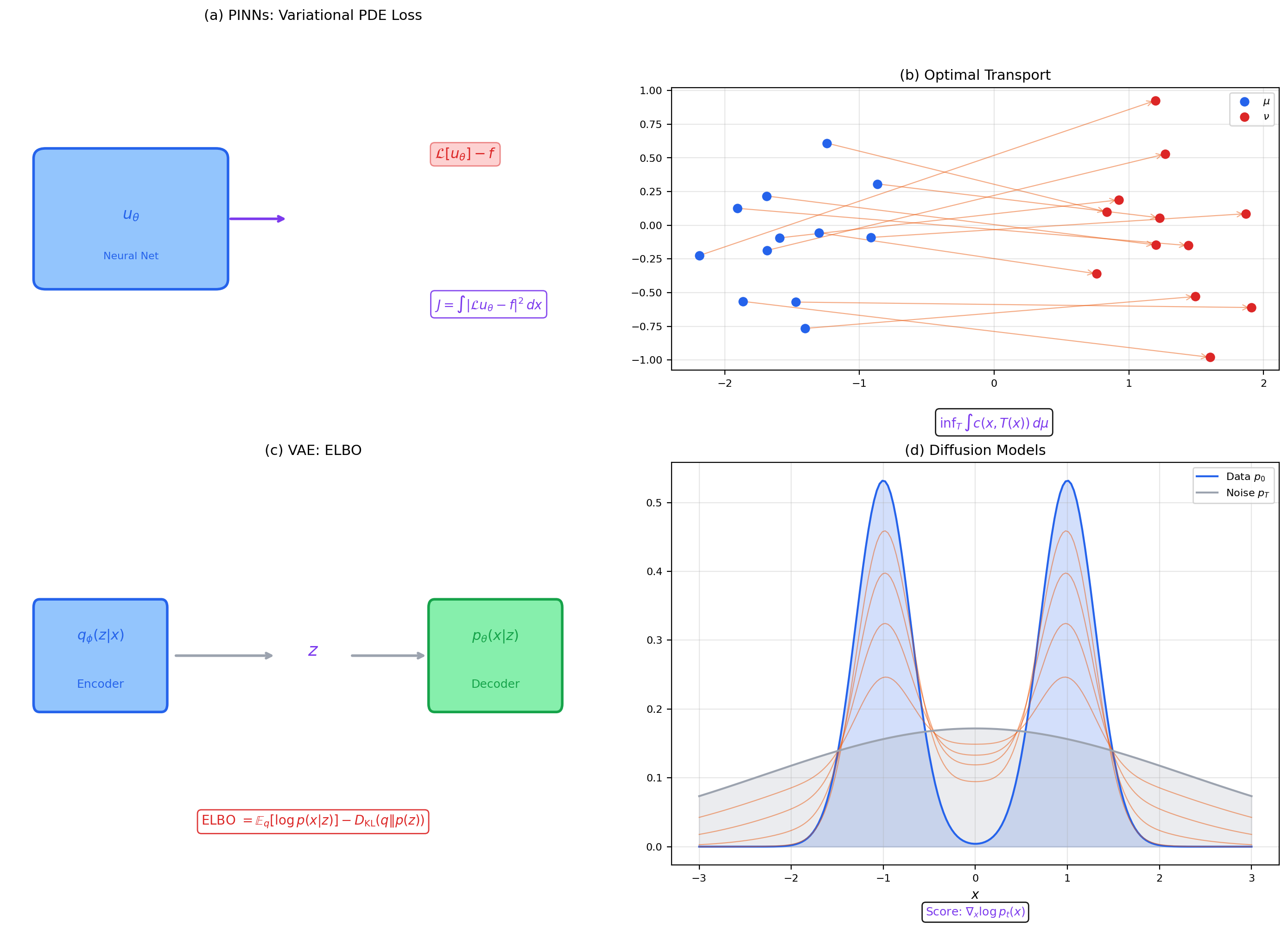
📝 Example 20 (Physics-Informed Neural Networks (PINNs))
A PINN parameterizes the solution of a PDE as a neural network and minimizes the variational loss
This is literally a calculus-of-variations problem: is a functional on the space of network functions. The Euler-Lagrange equation for recovers the PDE — the PINN finds an approximate solution by minimizing the variational residual. The direct method guarantees that a minimizer exists in (the Sobolev space), and the neural network approximates it.
📝 Example 21 (Optimal Transport)
The Monge-Kantorovich problem seeks the transport map minimizing the total cost . In its relaxed (Kantorovich) formulation, we minimize over transport plans :
The Wasserstein distance metrizes the space of probability measures. This is a variational problem over a function space — the direct method applies because the set of transport plans is weakly compact and the cost functional is lower semicontinuous.
📝 Example 22 (Variational Autoencoders (VAEs))
A VAE maximizes the evidence lower bound (ELBO):
This is a variational objective over the encoder and decoder . The name “variational” is literal: we are optimizing a functional over a family of distributions. The ELBO is related to the calculus of variations through the Euler-Lagrange equation for the optimal encoder, which yields the posterior .
📝 Example 23 (Diffusion Models)
Score-matching diffusion models minimize
where is the score network. This is a variational problem: minimize a functional over the space of score functions. The optimal score is the Euler-Lagrange solution. The connection to stochastic calculus (the reverse-time SDE) adds a layer of calculus-of-variations structure.
💡 Remark 10 (The Variational Principle in ML)
Across PINNs, optimal transport, VAEs, and diffusion models, the pattern is the same: define a functional on a function space, and minimize it. The calculus of variations provides the theoretical foundation — existence of minimizers (direct method), necessary conditions (Euler-Lagrange), sufficiency (second variation), and the functional-analytic setting (Sobolev spaces, Hilbert spaces). Understanding this machinery is not optional for serious ML research; it is the language in which the theory is written.
13. Computational Notes
The Euler-Lagrange equation can be solved numerically via finite differences or finite elements. Here is a minimal example for the Dirichlet energy minimization on with :
import numpy as np

# Finite difference discretization of -u'' = f on [0,1]
n = 100
h = 1.0 / (n + 1)
x = np.linspace(h, 1 - h, n)

# Stiffness matrix (tridiagonal)
A = (2 * np.eye(n) - np.eye(n, k=1) - np.eye(n, k=-1)) / h**2

# Right-hand side: f(x) = sin(pi*x)
f = np.sin(np.pi * x)

# Solve Au = f
u = np.linalg.solve(A, f)

# Exact solution: u(x) = sin(pi*x) / pi^2
u_exact = np.sin(np.pi * x) / np.pi**2
print(f"Max error: {np.max(np.abs(u - u_exact)):.2e}")
For the Rayleigh quotient iteration (finding eigenvalues variationally):
# Power method for the smallest eigenvalue of -u''
u = np.ones(n) / np.sqrt(n)  # initial guess
for _ in range(50):
    v = np.linalg.solve(A, u)       # apply A^{-1}
    lam = np.dot(u, v)              # Rayleigh quotient
    u = v / np.linalg.norm(v)       # normalize
print(f"λ₁ ≈ {1/lam:.6f} (exact: {np.pi**2:.6f})")
14. Track 8 Summary
The Functional Analysis Essentials track progressed through four levels of abstraction:
- Metric spaces — distance, completeness, compactness.
- Banach spaces — norms, bounded operators, the big four theorems.
- Hilbert spaces — inner products, projection, Riesz, spectral theory, RKHS.
- Calculus of variations — functionals, Euler-Lagrange, Sobolev spaces, direct method, Lax-Milgram.
Each level added one axiom and gained enormous power. The staircase is now complete.
15. Summary
| Element | Statement |
|---|---|
| Def. 1 | Functional: a map from a function space |
| Def. 2 | First variation: , the directional derivative of at in direction |
| Def. 3 | Second variation: , the second-order directional derivative |
| Def. 4 | Conjugate points and the Jacobi equation |
| Def. 5 | Weak derivative via integration by parts |
| Def. 6 | Sobolev spaces and |
| Def. 7 | Coercivity and weak lower semicontinuity |
| Def. 8 | Weak solution of a PDE |
| Def. 9 | Bilinear form — coercivity and boundedness |
| Def. 10 | Sturm-Liouville eigenvalue problem |
| Thm. 1 | Fundamental lemma of the calculus of variations |
| Thm. 2 | The Euler-Lagrange equation |
| Thm. 3 | Legendre’s necessary condition: |
| Thm. 4 | Jacobi’s sufficient condition: no conjugate points → minimum |
| Thm. 5 | is a Hilbert space |
| Thm. 6 | Poincaré inequality |
| Thm. 7 | Rellich-Kondrachov compactness (stated) |
| Thm. 8 | The direct method: coercive + w.l.s.c. → minimum attained |
| Thm. 9 | Lax-Milgram theorem |
| Thm. 10 | Variational characterization of eigenvalues |
| Thm. 11 | Min-max principle (Courant-Fischer) |
16. Closing Reflection
We have reached the summit.
Topic 32 is the 32nd and final topic on formalCalculus — the last node in a directed graph that began with epsilon-delta definitions and ends here, with the calculus of variations. Let us take a moment to see where we have been.
The journey through single-variable calculus (Topics 1–8) built the foundations: limits, continuity, derivatives, integrals, and Taylor series — the language in which all subsequent mathematics is written. Multivariable calculus (Topics 9–14) extended this machinery to : gradients, Jacobians, Hessians, multiple integrals, line integrals, surface integrals. Series and approximation (Topics 15–18) taught us to represent functions as infinite sums — power series, Fourier series, uniform convergence — and to quantify the quality of approximations. Ordinary differential equations (Topics 19–22) showed how derivatives drive dynamics: first-order equations, linear systems, stability theory, and numerical methods. Measure and integration (Topics 23–28) rebuilt the integral from the ground up: sigma-algebras, the Lebesgue integral, spaces, the Radon-Nikodym theorem — replacing the Riemann integral with a theory powerful enough for modern analysis. And functional analysis (Topics 29–32, this track) assembled the abstract framework: metric spaces, normed and Banach spaces, inner-product and Hilbert spaces, and finally the calculus of variations.
At each level, the pattern was the same: add one axiom, gain an enormous amount of power. A metric gives completeness and fixed-point theorems. A norm gives bounded operators and the big four theorems. An inner product gives projection, Riesz representation, and spectral decomposition. And the variational perspective — optimizing functionals on function spaces — gives the Euler-Lagrange equation, the direct method for existence, Sobolev spaces, and the Lax-Milgram theorem.
These are not just mathematical curiosities. They are the foundations of modern machine learning. Every gradient descent step invokes the calculus. Every loss function is a functional. Every regularized objective lives in a Sobolev space. Every kernel method operates in a reproducing kernel Hilbert space. Every PINN solves a variational problem. Every diffusion model minimizes a score-matching loss that is a functional over function spaces.
The reader who has worked through all 32 topics now has the rigorous calculus and analysis machinery that formalML assumes. The path forward is clear: Lagrangian duality, information geometry, optimization theory, spectral methods, generative modeling. The foundations are laid. The mathematics is yours.
Connections & Further Reading
Prerequisites — topics you need first
Inner Product & Hilbert Spaces
The projection theorem, Riesz representation, and spectral theory from Topic 31 provide the Hilbert-space infrastructure on which the direct method and Lax-Milgram theorem operate.
Mean Value Theorem & Taylor Expansion
Taylor expansion underlies the first and second variation — the Euler-Lagrange equation is the function-space analog of setting the first derivative to zero.
Metric Spaces & Topology
Compactness and completeness from Topic 29 (Arzelà-Ascoli, Bolzano-Weierstrass) reappear in the direct method as weak compactness in Sobolev spaces.
Normed & Banach Spaces
Sobolev spaces are Banach spaces (and Hilbert spaces for p=2). The open mapping theorem and bounded inverse theorem from Topic 30 underlie the well-posedness of variational problems.
Line Integrals & Conservative Fields
Geodesics are extremals of the arc-length functional — a line integral whose Euler-Lagrange equation yields the geodesic equation.
Surface Integrals & the Divergence Theorem
The Euler-Lagrange equation for area-minimizing surfaces connects to minimal surfaces and the divergence theorem.
Approximation Theory
Best approximation in function spaces is a variational problem. The Weierstrass theorem guarantees existence; the direct method provides the general principle.
On to formalStatistics — where this calculus powers inference
On to formalML — where this calculus powers ML
Lagrangian Duality
The Euler-Lagrange equation is the infinite-dimensional prototype for first-order optimality conditions. Lagrangian duality generalizes constrained variational problems to convex optimization.
Information Geometry
Geodesics on statistical manifolds are calculus-of-variations problems with the Fisher information metric as the Lagrangian.
Gradient Descent
The direct method provides the functional-analytic foundation for the existence of minimizers. Gradient descent in function spaces (gradient flow) is a continuous-time variational principle.
References
- book Dacorogna (2015). Introduction to the Calculus of Variations Primary reference for the direct method and Sobolev spaces
- book Gelfand & Fomin (1963). Calculus of Variations Classical reference for Euler-Lagrange derivation and classical examples
- book Brezis (2011). Functional Analysis, Sobolev Spaces and Partial Differential Equations Sobolev spaces and Lax-Milgram theorem
- book Evans (2010). Partial Differential Equations Weak solutions, Sobolev embedding theorems
- paper Raissi, Perdikaris & Karniadakis (2019). “Physics-Informed Neural Networks” Foundational PINN paper