Surface Integrals & the Divergence Theorem
Integrating functions and vector fields over surfaces in ℝ³ — flux through oriented surfaces, the 3D curl and divergence, Stokes' theorem generalizing Green's from 2D to 3D, and the divergence theorem relating boundary flux to interior divergence.
Abstract. Surface integrals extend integration from curves to two-dimensional surfaces embedded in ℝ³. Given a parameterized surface S defined by r(u,v) for (u,v) in a parameter domain D*, the tangent vectors r_u and r_v span the tangent plane at each point, and their cross product r_u × r_v yields the normal vector whose magnitude is the surface area element dS = ‖r_u × r_v‖ du dv. For a scalar function f, the scalar surface integral ∬_S f dS = ∬_{D*} f(r(u,v)) ‖r_u × r_v‖ du dv sums f over S weighted by area. For a vector field F, the flux integral ∬_S F · dS = ∬_{D*} F(r(u,v)) · (r_u × r_v) du dv measures the net flow of F through the oriented surface. These constructions culminate in two fundamental theorems. Stokes' theorem ∮_C F · dr = ∬_S (∇ × F) · dS generalizes Green's theorem from 2D to 3D: the circulation of F around the boundary curve C of a surface S equals the flux of the curl ∇ × F through S. The divergence theorem (Gauss's theorem) ∬_S F · dS = ∭_E ∇ · F dV relates the net outward flux of F through a closed surface S to the total divergence of F in the enclosed volume E. Together, these theorems unify Green's theorem, the Gradient Theorem, and the Fundamental Theorem of Calculus under a single framework — the generalized Stokes' theorem ∫_M dω = ∫_{∂M} ω — connecting boundary integrals to interior derivatives at every dimension. In machine learning, the divergence theorem appears in conservation laws for gradient flow trajectories, in Stein's identity (the foundation of Stein variational gradient descent), in physics-informed neural networks enforcing PDE constraints, and in the flow-matching framework for generative models where the continuity equation ∂_t p + ∇ · (p v) = 0 governs density evolution under a learned velocity field.
1. Overview & Motivation
You’re building a flow-matching generative model. The core idea: learn a velocity field that transforms a simple base distribution (say, a Gaussian) into your target data distribution over time . The evolving probability density obeys the continuity equation:
This equation says that probability is neither created nor destroyed — it flows. But how do we verify that no probability mass leaks through the boundaries of a region? We integrate the continuity equation over a volume and apply the divergence theorem:
The left side is the rate of change of total probability inside . The right side is the net flux of the probability current through the boundary surface . The divergence theorem converts the volume integral of into this boundary flux — verifying mass conservation without tracking individual particles.
This is why we need surface integrals. They measure flow through surfaces — the net amount of a vector quantity passing through a two-dimensional membrane embedded in . The divergence theorem then connects that surface measurement to what happens in the interior. Together with Stokes’ theorem (which connects surface integrals to line integrals around the boundary), these results complete the hierarchy that started with the Fundamental Theorem of Calculus: interior derivatives determine boundary integrals, at every dimension.
2. Parameterized Surfaces & the Area Element
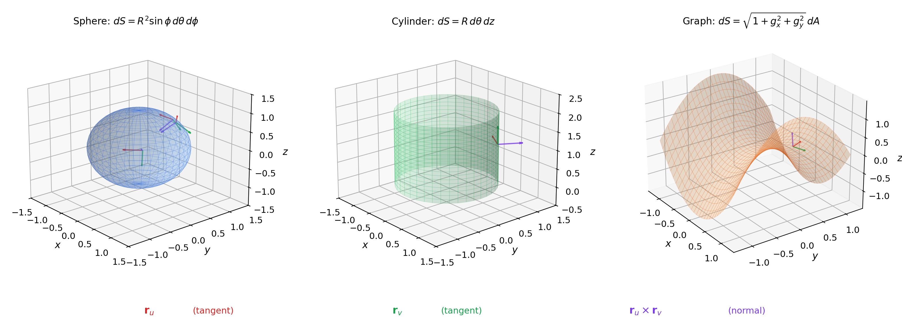
A surface in is the two-dimensional analog of a curve. Where a curve is traced by one parameter , a surface is swept out by two parameters . At each point, the partial derivatives and are tangent vectors that span the tangent plane. Their cross product is perpendicular to the surface — it is the normal vector — and its magnitude gives the area of the infinitesimal parallelogram spanned by and . This magnitude is the surface area element .
The connection to the Jacobian (Topic 14) is precise: the parameterization is a map from a 2D parameter domain to 3D space. Its Jacobian matrix is . In the change-of-variables theorem, the scaling factor was , the absolute value of the determinant of a square Jacobian. Here the Jacobian is not square, so we use the Gram determinant instead — and this turns out to equal .
📐 Definition 1 (Parameterized Surface)
A parameterized surface in is a function , where is a bounded, closed region (the parameter domain). We write .
The surface is regular (or smooth) if the cross product for all in the interior of . This ensures the tangent plane is well-defined at every point — the two tangent vectors are linearly independent, and the surface has no cusps or self-intersections locally.
📐 Definition 2 (Cross Product)
For vectors and in , the cross product is:
Equivalently, using the determinant mnemonic:
Key properties:
- Orthogonality: and — the cross product is perpendicular to both factors.
- Area: — the magnitude equals the area of the parallelogram spanned by and .
- Anti-commutativity: — swapping the factors reverses the direction.
📐 Definition 3 (Surface Area Element)
For a regular parameterized surface , the surface area element is:
The surface area of is:
The factor is the area of the infinitesimal parallelogram spanned by the tangent vectors — it measures how much the parameterization stretches area at each point.
💡 Remark 1 (Connection to the Jacobian)
The Jacobian matrix of the parameterization is the matrix , with columns and . The Gram matrix is the matrix:
By the Lagrange identity:
So . This is the natural generalization of the 1D Jacobian from Topic 14: when the map goes from to with , the area scaling factor is .
📝 Example 1 (Sphere of Radius R)
Parameterize the sphere of radius using spherical coordinates with (azimuthal) and (polar):
The tangent vectors are:
We compute the cross product component by component:
The -component: .
The -component: .
The -component: .
So . Wait — let us be more careful. Factoring:
The vector is the outward unit normal on the sphere, so . (The negative sign means this particular parameterization gives the inward normal; we can reverse it by swapping the order of the cross product.) The magnitude is:
The surface area is:
📝 Example 2 (Cylinder)
The cylinder of radius and height is parameterized by:
The tangent vectors are and . The cross product is:
with magnitude . The lateral surface area is:
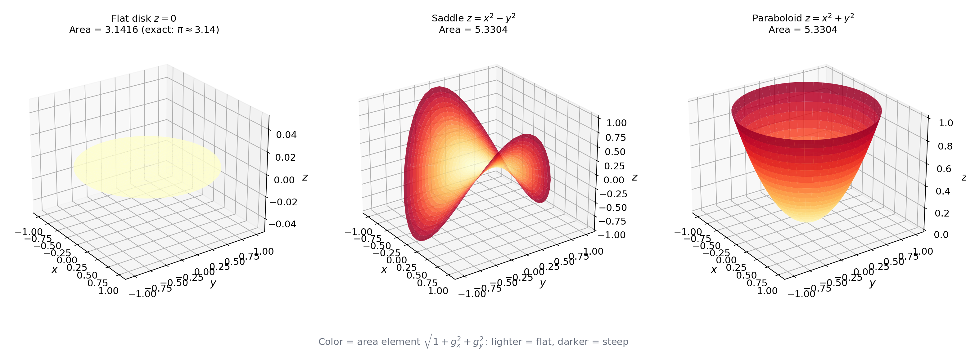
📝 Example 3 (Graph Surface z = g(x,y))
A surface defined as the graph of a function over a region has the natural parameterization . The tangent vectors are:
The cross product is:
with magnitude . So the surface area element for a graph is:
where . This is a formula worth memorizing: for a graph surface, the area element is the Euclidean area scaled by the factor , which measures how much the surface tilts away from horizontal.
🔷 Proposition 1 (Parameterization Independence)
The surface area is independent of the parameterization. If is a reparameterization via a diffeomorphism , then computed via equals computed via .
Proof.
By the chain rule, the Jacobian of is , where is the Jacobian of the reparameterization. The tangent vectors transform as:
Taking magnitudes and applying the change of variables theorem (Topic 14):
The from the cross product formula is absorbed by the from the change-of-variables substitution, leaving the original integral.
Click on the parameter domain (left) to select a point. Drag to rotate the 3D view (right).
3. Scalar Surface Integrals
The scalar surface integral sums the values of a function over a surface , weighted by the surface area element. This is the 2D analog of the scalar line integral from Topic 15 — where the wire becomes a thin shell.
Imagine a thin hemispherical dome with a density that varies from point to point — thicker at the base, thinner at the top. The total mass is , where is the density (mass per unit area) at each point on the surface. We weight by rather than because the physical mass depends on the geometry of the surface, not on the parameterization. Just as a wire’s mass depended on arc length, a shell’s mass depends on surface area.
📐 Definition 4 (Scalar Surface Integral)
Let be a regular parameterized surface , and let be continuous. The scalar surface integral of over is:
This is a double Riemann integral (Topic 13) of the composite function over the parameter domain .
💡 Remark 2 (Parameterization Independence)
The scalar surface integral is independent of the parameterization, including orientation. The proof is identical to Proposition 1: the from the area element cancels with the from the change of variables in the double integral. The absolute value ensures the result holds regardless of whether the reparameterization preserves or reverses orientation.
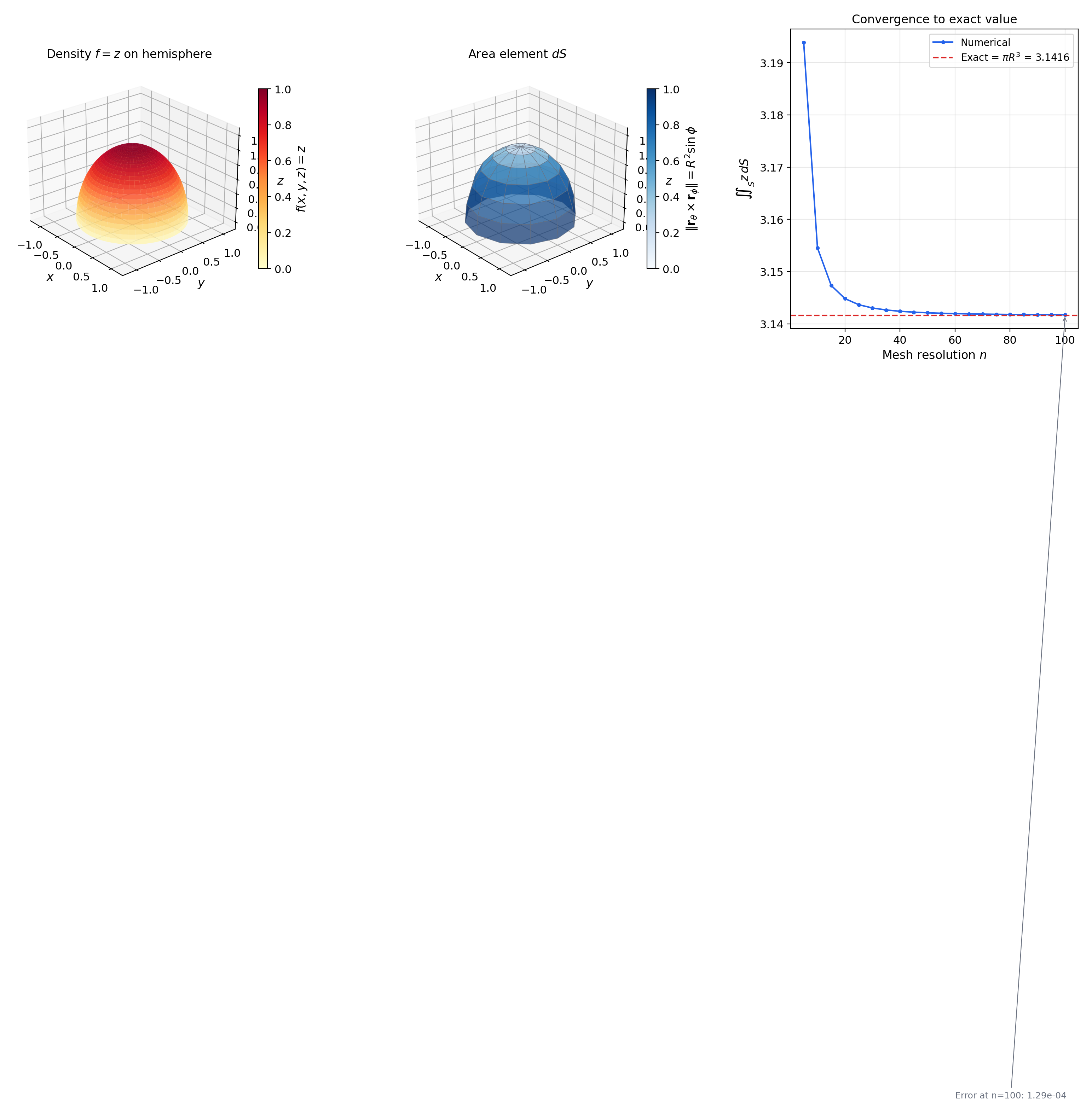
📝 Example 4 (Mass of a Hemispherical Shell)
Let be the upper hemisphere of radius (i.e., with ) and let be the density. From Example 1, we use the spherical parameterization with (upper hemisphere only) and . On the sphere, , so:
The inner integral: .
So .
📝 Example 5 (Average Temperature on a Surface)
The average value of over is:
directly analogous to from single-variable calculus (Topic 7) and for curves (Topic 15, Example 5). For the hemispherical shell with , the average height is — the average height on the hemisphere is half the radius, which matches geometric intuition (the hemisphere is “top-heavy” in the -direction but the area element weights the equatorial region more heavily).
4. Oriented Surfaces & Flux Integrals
We now move from scalar functions to vector fields. The question changes from “how much density sits on the surface?” to “how much fluid flows through the surface?”
Think of as the velocity field of a fluid and as a fishing net stretched across the flow. At each point on the net, only the component of normal to the surface passes through — the tangential component slides along the net without crossing it. The flux is the integral of over the surface: the total rate at which fluid passes through from one side to the other.
To define flux, we need a consistent notion of “which side is which” — a choice of orientation, meaning a continuous choice of unit normal vector at each point.
📐 Definition 5 (Oriented Surface)
A surface is orientable if it admits a continuous unit normal vector field with and perpendicular to the tangent plane at every point. An oriented surface is an orientable surface together with a specific choice of .
For a parameterized surface, the two orientations correspond to and .
Not every surface is orientable. The Mobius strip is the classic counterexample: if you start with a normal vector and slide it continuously around the strip, it returns pointing the opposite way. There is no globally consistent choice of “inside” and “outside.”
💡 Remark 3 (Orientation Conventions)
Two standard conventions govern orientation:
-
Closed surfaces (surfaces that enclose a volume, like a sphere or cube): the outward-pointing normal is the positive orientation. Flux with the outward normal measures net outflow.
-
Surfaces with boundary (for Stokes’ theorem): the right-hand rule determines the orientation. If you curl the fingers of your right hand in the direction of traversal along the boundary curve , your thumb points in the direction of . Equivalently: walking along with pointing up from your head, the surface is on your left.
📐 Definition 6 (Flux Integral)
Let be an oriented surface parameterized by (with the orientation given by ), and let be a continuous vector field. The flux integral (or surface integral of a vector field) is:
Equivalently, writing :
The flux measures the net flow of through in the direction of . Positive flux means net flow in the direction; negative flux means net flow opposite to .
📝 Example 6 (Flux Through a Hemisphere)
Let (a vertical field, stronger at greater heights) and let be the upper hemisphere of the unit sphere () with the outward normal. From Example 1, .
Since we want the outward normal, we use . On the sphere, , so .
The flux is:
With the substitution , :
📝 Example 7 (Flux of the Position Field Through a Sphere)
Let — the position (or radial) field — and let be the sphere of radius with the outward normal. On the sphere, , so:
The normal component of is the constant on the entire sphere. The flux is:
We can verify this using the divergence theorem (Theorem 3, Section 7): , so . The two sides match — this is the divergence theorem at work.
💡 Remark 4 (Orientation Reversal)
Reversing the orientation of — replacing by — negates the flux integral:
This is the surface analog of the line integral identity from Topic 15, Remark 2. The scalar surface integral is orientation-independent (it uses , which is always positive), but the flux integral is orientation-sensitive (it uses directly, including its sign).
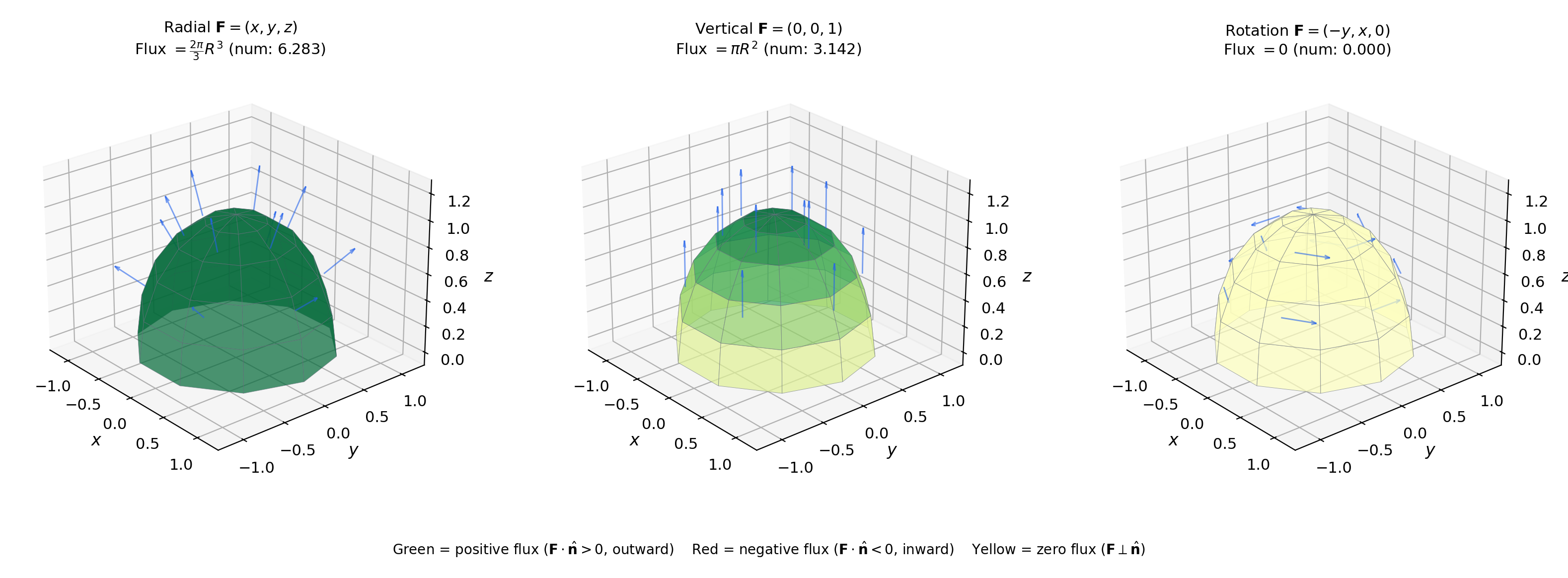
Drag to rotate. Green = positive flux (outward), Red = negative flux (inward).
5. The 3D Curl and Divergence
Before stating Stokes’ theorem and the divergence theorem, we need the two differential operators that generalize the 2D curl from Topic 15 to three dimensions.
The geometric intuition is direct. The curl of a vector field at a point measures the rotation — the axis and angular velocity of the infinitesimal “paddlewheel” that would spin. The divergence measures the source strength — how much is “spreading out” or “converging” at that point. If is a fluid velocity field, points along the local rotation axis, and is the rate of volume expansion per unit volume.
📐 Definition 7 (3D Curl)
For a vector field , the curl of is:
Using the determinant mnemonic:
The -component of is — exactly the 2D curl from Topic 15, Definition 9. The 3D curl extends the 2D curl by adding components for rotation about the - and -axes.
📐 Definition 8 (3D Divergence)
For a vector field , the divergence of is the scalar field:
The divergence is the “scalar product” of the formal vector with . It measures the net outflow per unit volume at each point.
🔷 Proposition 2 (Divergence as Infinitesimal Flux)
Let be at a point . Let be the ball of radius centered at and its boundary sphere (with outward normal). Then:
The divergence is the flux per unit volume in the limit of infinitesimally small enclosing surfaces.
Proof.
By the divergence theorem (Theorem 3, which we will prove in Section 7), . By the Mean Value Theorem for triple integrals (Topic 13), there exists such that:
Dividing by the volume and taking : as , , and continuity of gives .
🔷 Proposition 3 (Curl as Infinitesimal Circulation (3D))
Let be at a point , and let be a unit vector. Let be the circle of radius centered at in the plane perpendicular to , oriented by the right-hand rule. Then:
The component of the curl along is the circulation per unit area in the plane perpendicular to , in the limit of infinitesimally small loops. This generalizes Topic 15, Proposition 2 from 2D (where always) to arbitrary directions in 3D.
🔷 Theorem 1 (Key Vector Identities)
Let be a scalar field and a vector field on an open domain in . Then:
-
— the curl of a gradient is always zero.
-
— the divergence of a curl is always zero.
-
— the curl-curl identity, where is the vector Laplacian (Laplacian applied component-wise).
Identity (1) says gradient fields are curl-free — this is the 3D version of the exactness condition from Topic 15. Identity (2) says curl fields are divergence-free. Together, they form an exact sequence:
where the composition of any two consecutive arrows is zero. In the language of differential forms, this is the de Rham complex with (→ Smooth Manifolds on formalML).
📝 Example 8 (Computing Curl and Divergence)
Let . We compute:
The curl vanishes because — it is a gradient field, and Identity (1) from Theorem 1 guarantees .
The divergence is . This field is both curl-free and divergence-free — it has no rotation and no sources or sinks.
📝 Example 9 (Non-Trivial Curl)
Let — the 3D extension of the rotation field from Topic 15.
The curl is , pointing in the direction with magnitude 2. The -component is , exactly the 2D curl from Topic 15, Example 15. The 3D curl encodes the same rotation information, plus the fact that the rotation axis is vertical.
The divergence is — rotation without expansion.

6. Stokes’ Theorem
Green’s theorem (Topic 15, Theorem 5) says — the circulation around a closed curve equals the integral of the curl over the enclosed region . This worked in 2D because bounds a flat region in the plane.
Stokes’ theorem is the 3D generalization. The “enclosed region” is now a surface bounded by the curve , and the “integral of the curl” becomes the flux of the curl through . The flat 2D region becomes a potentially curved surface — the boundary is still a curve, but the “inside” can be any surface spanning that curve.
🔷 Theorem 2 (Stokes' Theorem)
Let be an oriented, piecewise-smooth surface in bounded by a simple, closed, piecewise-smooth curve , with orientation induced by the right-hand rule. Let be a vector field on an open region containing . Then:
The circulation of around the boundary equals the flux of the curl through the surface .
Proof.
We prove Stokes’ theorem for the case where is the graph of a function over a region . The general case follows by decomposing an arbitrary surface into graph patches using a partition of unity.
Setup. Parameterize as for . The boundary curve lies above the boundary . If is parameterized by for , then is parameterized by .
Left side (line integral). We compute . On , (by the chain rule), so:
where all functions are evaluated at . This is now a 2D line integral around .
Right side (surface integral). We compute . From Example 3, . Writing , the flux of the curl is:
where all partial derivatives of , , are evaluated at .
Showing equality via Green’s theorem. We apply Green’s theorem (Topic 15, Theorem 5) to the 2D line integral:
We now expand the integrand on the right. We must use the chain rule carefully, because , , depend on .
Expanding :
so .
Expanding :
so .
Subtracting. Since (by regularity), the and terms cancel. The terms also cancel. We are left with:
Rearranging:
Wait — let us verify. We have . Grouping by the factors:
This is exactly .
So by Green’s theorem:
For a general oriented surface that is not a single graph, we decompose into graph patches using a partition of unity. The interior boundary contributions from adjacent patches cancel (their normals point in opposite directions along the shared edge), leaving only the exterior boundary .
📝 Example 10 (Verifying Stokes' on a Hemisphere)
Let and let be the upper hemisphere of the unit sphere, bounded by : the unit circle in the -plane.
Line integral. The unit circle is for , traversed counterclockwise. Then and :
Surface integral. From Example 9, . The flux of through the upper hemisphere with outward normal: using :
Both sides equal . Stokes’ theorem confirmed.
📝 Example 11 (Stokes' Theorem as a Computation Tool)
Compute where and is the triangle with vertices , , , oriented counterclockwise when viewed from the direction of the outward normal.
Strategy: computing the line integral directly would require parameterizing three edges and adding three integrals. Instead, we use Stokes’ theorem with the flat triangular surface spanning .
The triangle lies in the plane , which we can write as . So and , and (pointing outward, since the components are all positive — this is the outward normal to the plane ).
The curl is:
The flux of the curl through the triangle:
On the plane : . So:
where is the projection of the triangle onto the -plane: the triangle with vertices , , . Its area is . Therefore:
💡 Remark 5 (Surface Independence)
Stokes’ theorem implies that if two oriented surfaces and share the same boundary curve (with compatible orientations), then:
The flux of the curl depends only on the boundary, not on which surface spans it. In Example 10, we could replace the hemisphere with any surface bounded by the unit circle — a flat disk, a paraboloid, a cone — and the curl flux would still be .
This is the surface analog of path independence for conservative fields: for a curl field (one of the form ), the flux integral is “surface-independent” in the same way that a gradient field’s line integral is “path-independent.”
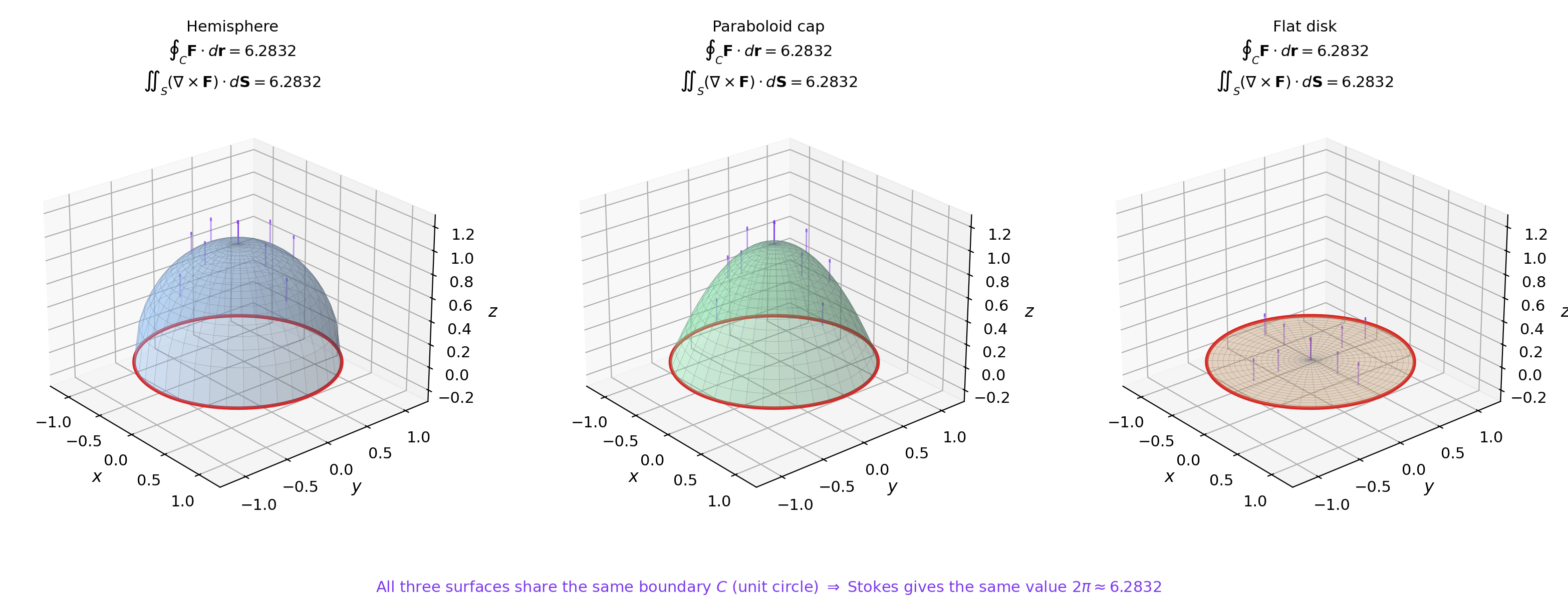
Stokes' theorem: ∮C F·dr = ∬S (∇×F)·dS. Drag to rotate.
7. The Divergence Theorem
The divergence theorem is the 3D analog of the 2D divergence form of Green’s theorem. It relates the flux of a vector field through a closed surface to the integral of the divergence over the enclosed volume.
The geometric intuition is the same telescoping argument that underlies the Fundamental Theorem of Calculus. Chop the volume into tiny cubes. Each tiny cube contributes its flux through its six faces. But adjacent cubes share faces, and the flux through a shared face is counted out of one cube and in to its neighbor — these contributions cancel. The only faces that survive are those on the outer boundary . So the total flux through equals the sum of the divergences (the infinitesimal net outflows) over all the tiny cubes — which in the limit is .
🔷 Theorem 3 (The Divergence Theorem (Gauss's Theorem))
Let be a bounded region with piecewise-smooth boundary surface , oriented with the outward-pointing normal. Let be a vector field on an open region containing . Then:
The net outward flux of through the closed surface equals the total divergence of in the enclosed volume .
Proof.
We prove the divergence theorem for regions that are simultaneously Type I, Type II, and Type III — that is, regions that can be described as bounded above and below by graphs in each coordinate direction. It suffices to show:
and then add all three. We prove the third identity; the first two are analogous.
Proof of . Let be a Type I region in the -direction:
where is the projection of onto the -plane, and is the bottom surface, is the top surface.
Right side (volume integral). By Fubini’s theorem (Topic 13):
The inner integral is evaluated by the Fundamental Theorem of Calculus.
Left side (surface integral). The boundary consists of three pieces:
-
Top surface : with upward (outward) normal. Parameterized as , so . The -component of the flux uses only the -component of , which is . So .
-
Bottom surface : with downward (outward) normal. The outward normal points downward, so (we reverse the cross product). The -component is . So .
-
Lateral surface : the vertical sides. On vertical surfaces, the normal is horizontal — the -component of is zero. So .
Adding all three pieces:
This matches the volume integral computed above.
The proofs for the and components are identical, using the Type II and Type III descriptions of respectively. Adding all three:
For general regions that are not simultaneously Type I/II/III, we decompose into finitely many subregions , each of which is Type I/II/III. The divergence theorem holds on each piece. The flux contributions from shared interior faces cancel (they have opposite outward normals on adjacent subregions), leaving only the flux through the external boundary .
📝 Example 12 (Verification on a Cube)
Let and let be the unit cube.
Divergence: .
Volume integral:
By symmetry (each variable contributes equally), this is .
Surface integral (direct computation). The cube has six faces. On : , , integral . On : , , integral . By symmetry, the -faces contribute and the -faces contribute .
Total flux: .
Both sides equal 3. Divergence theorem confirmed.
📝 Example 13 (The Inverse-Square Field)
Let — the gravitational/electrostatic field of a point source at the origin.
Away from the origin, . We can verify this by direct computation:
Summing the three components: .
On a sphere of radius centered at the origin, and . The flux is:
The flux is regardless of . If the divergence theorem applied to the ball containing the origin, we would get , contradicting the nonzero flux. The resolution: is not at the origin. The divergence theorem does not apply to regions containing the singularity. In the distributional sense, , where is the Dirac delta — the “divergence” is zero everywhere except at the origin, where it is infinite in a precise measure-theoretic sense.
💡 Remark 6 (Conservation Laws)
The divergence theorem is the mathematical engine behind conservation laws. Consider a quantity with density that flows with flux density . If the quantity is conserved (neither created nor destroyed), the amount in any region changes only by flow through the boundary:
Applying the divergence theorem to the right side and moving the time derivative inside the integral (assuming sufficient smoothness):
Since this holds for every region , the integrands must be equal pointwise:
This is the continuity equation — the local form of conservation. For a fluid with density and velocity , , giving , which is exactly the equation we started with in Section 1.
💡 Remark 7 (The Generalized Stokes' Theorem)
The Fundamental Theorem of Calculus, the Gradient Theorem, Green’s theorem, Stokes’ theorem, and the divergence theorem are all instances of a single result — the generalized Stokes’ theorem:
where is an oriented manifold with boundary , is a differential form, and is the exterior derivative.
| Dimension of | Theorem | |||
|---|---|---|---|---|
| 1 (interval) | (0-form) | FTC: | ||
| 1 (curve) | Curve | Endpoints | (0-form) | Gradient Theorem: |
| 2 (region) | Region | Curve | 1-form | Green’s theorem |
| 2 (surface) | Surface | Curve | 1-form | Stokes’ theorem |
| 3 (volume) | Volume | Surface | 2-form | Divergence theorem |
In every case: integrating a derivative () over the interior equals integrating the original () over the boundary. The exterior derivative unifies the gradient, curl, and divergence as the same operation on forms of different degrees.
This unification is the starting point for differential geometry and the theory of integration on manifolds — see Smooth Manifolds on formalML for the full treatment.
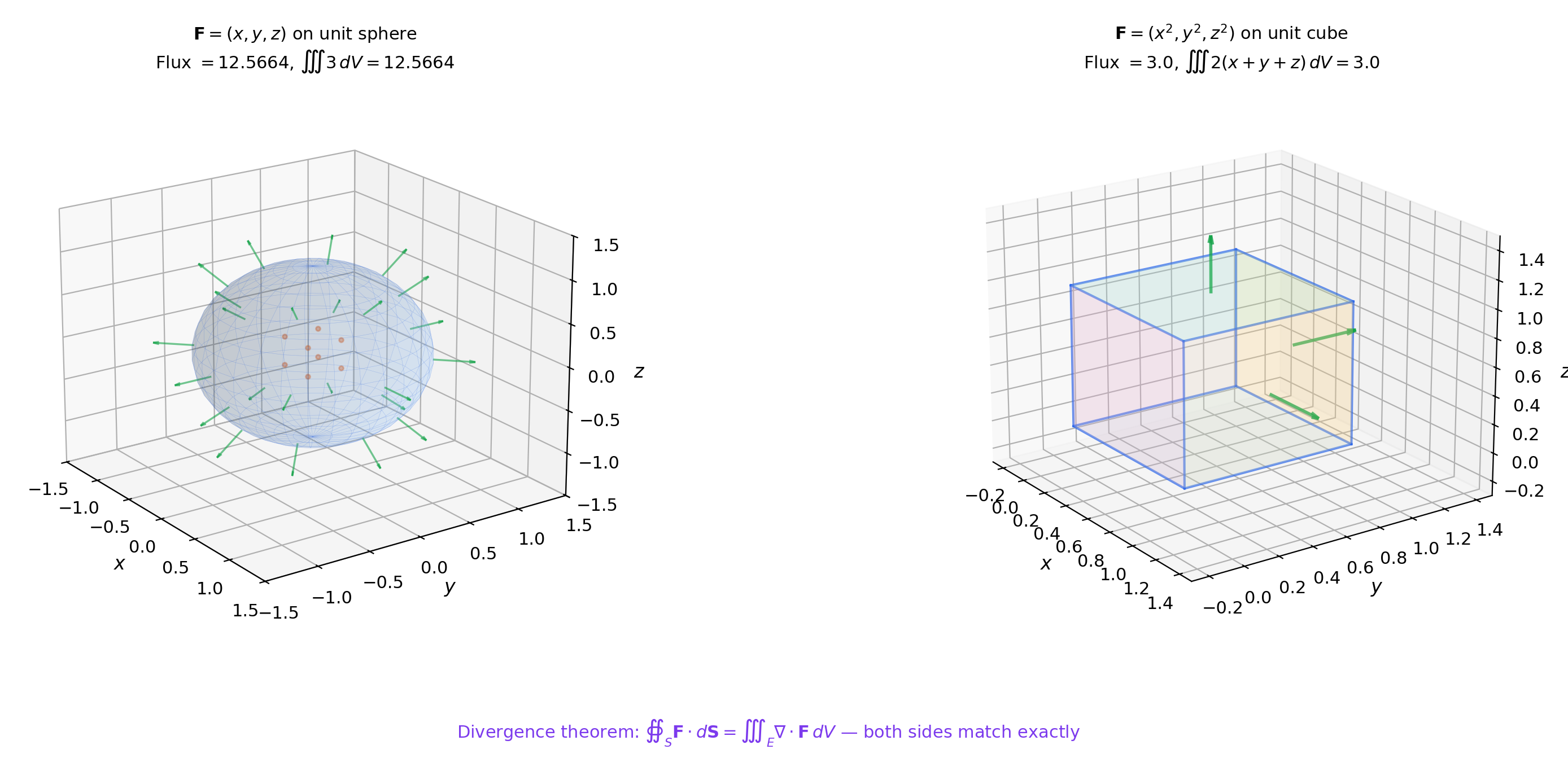
Divergence theorem: ∬S F·dS = ∭E ∇·F dV. Drag to rotate.
8. Graphs, Applications & Computation
For surfaces defined as graphs , the formulas simplify considerably. These are the most common surfaces in applications, and the simplified formulas are worth isolating.
🔷 Proposition 4 (Surface Integrals over a Graph)
Let be the graph of for , and let . Then:
Scalar integral:
Flux integral (with upward-pointing normal):
where all functions are evaluated at . This follows from (Example 3).
📝 Example 14 (Area of a Saddle Surface)
Compute the surface area of over the unit disk .
We have , , so in polar coordinates.
The inner integral: let , , so :
So .
(Note: the saddle surface warps significantly over the unit disk — its area is nearly 70% larger than the flat disk’s area of .)
📝 Example 15 (Flux via the Divergence Theorem)
Compute the flux of through the unit sphere .
Direct computation would require parameterizing the sphere and evaluating a complicated surface integral. Instead, we use the divergence theorem:
Converting to spherical coordinates (, , ) with :
Evaluating each factor: , , .
9. Computational Notes
In practice, surface integrals are computed by reducing to double integrals over the parameter domain, then applying numerical quadrature. Here are the key patterns.
Scalar surface integral:
import numpy as np
from scipy.integrate import dblquad

def scalar_surface_integral(f, r, r_u, r_v, u_bounds, v_bounds):
    """Compute ∬_S f dS via parameterization."""
    def integrand(v, u):
        point = r(u, v)
        cross = np.cross(r_u(u, v), r_v(u, v))
        return f(*point) * np.linalg.norm(cross)
    result, _ = dblquad(integrand, *u_bounds,
                        lambda u: v_bounds[0], lambda u: v_bounds[1])
    return result
Flux integral:
def flux_integral(F, r, r_u, r_v, u_bounds, v_bounds):
    """Compute ∬_S F · dS via parameterization."""
    def integrand(v, u):
        point = r(u, v)
        F_val = np.array(F(*point))
        cross = np.cross(r_u(u, v), r_v(u, v))
        return np.dot(F_val, cross)
    result, _ = dblquad(integrand, *u_bounds,
                        lambda u: v_bounds[0], lambda u: v_bounds[1])
    return result
Numerical curl and divergence:
def curl_3d(F, x, y, z, h=1e-7):
    """Compute ∇ × F at (x, y, z) via central differences."""
    Px, Qx, Rx = F(x + h, y, z)
    Pmx, Qmx, Rmx = F(x - h, y, z)
    Py, Qy, Ry = F(x, y + h, z)
    Pmy, Qmy, Rmy = F(x, y - h, z)
    Pz, Qz, Rz = F(x, y, z + h)
    Pmz, Qmz, Rmz = F(x, y, z - h)
    dRdy = (Ry - Rmy) / (2 * h)
    dQdz = (Qz - Qmz) / (2 * h)
    dPdz = (Pz - Pmz) / (2 * h)
    dRdx = (Rx - Rmx) / (2 * h)
    dQdx = (Qx - Qmx) / (2 * h)
    dPdy = (Py - Pmy) / (2 * h)
    return (dRdy - dQdz, dPdz - dRdx, dQdx - dPdy)

def divergence_3d(F, x, y, z, h=1e-7):
    """Compute ∇ · F at (x, y, z) via central differences."""
    dPdx = (F(x + h, y, z)[0] - F(x - h, y, z)[0]) / (2 * h)
    dQdy = (F(x, y + h, z)[1] - F(x, y - h, z)[1]) / (2 * h)
    dRdz = (F(x, y, z + h)[2] - F(x, y, z - h)[2]) / (2 * h)
    return dPdx + dQdy + dRdz
Verifying Stokes’ theorem numerically:
from scipy.integrate import quad

# F = (-y, x, 0), hemisphere bounded by unit circle
# Line integral around unit circle
def stokes_line(t):
    F = (-np.sin(t), np.cos(t), 0)
    dr = (-np.sin(t), np.cos(t), 0)
    return sum(f * d for f, d in zip(F, dr))

circulation, _ = quad(stokes_line, 0, 2 * np.pi)  # → 2π

# Surface integral of curl through hemisphere
def stokes_surface(phi, theta):
    # curl F = (0, 0, 2), outward normal on hemisphere
    sin_phi = np.sin(phi)
    cos_phi = np.cos(phi)
    curl_dot_n = 2 * sin_phi * cos_phi  # (0,0,2) · n̂ * |r_θ × r_φ|
    return curl_dot_n

curl_flux, _ = dblquad(stokes_surface, 0, 2 * np.pi,
                        0, np.pi / 2)  # → 2π
Verifying the divergence theorem numerically:
# F = (x², y², z²) on unit cube [0,1]³
from scipy.integrate import tplquad

# Volume integral of divergence
div_vol, _ = tplquad(
    lambda z, y, x: 2*x + 2*y + 2*z,
    0, 1, 0, 1, 0, 1
)  # → 3.0

# Flux through each face (computed analytically: 3.0)
# Face x=1: ∫∫ 1 dy dz = 1, face x=0: 0
# Face y=1: ∫∫ 1 dx dz = 1, face y=0: 0
# Face z=1: ∫∫ 1 dx dy = 1, face z=0: 0
# Total flux = 3.0
10. Connections to ML
Surface integrals and the divergence theorem are not abstract curiosities — they are the mathematical backbone of several active areas in modern machine learning.
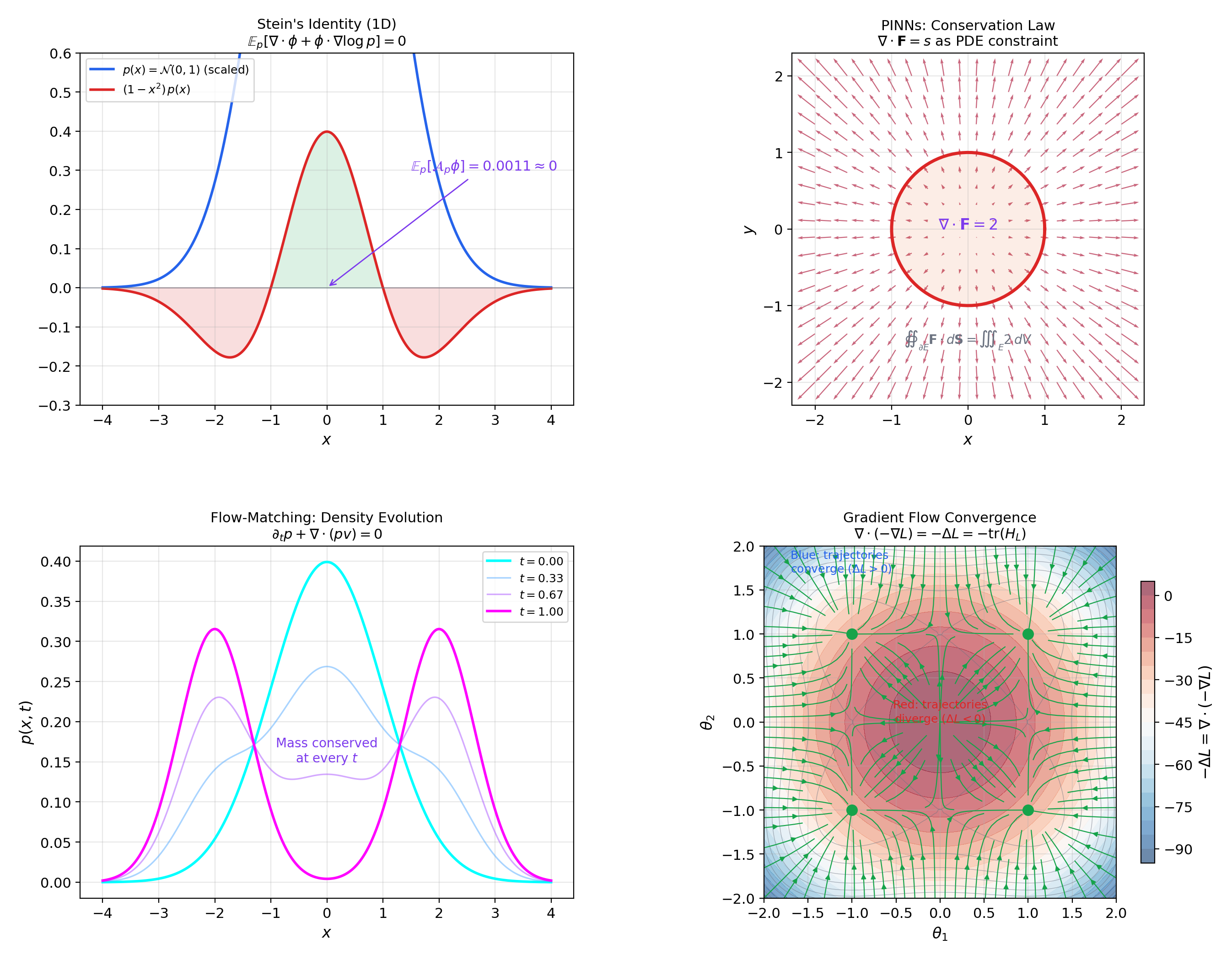
10.1 Stein’s Identity and SVGD
The divergence theorem yields one of the most powerful tools in computational statistics: Stein’s identity. Let be a smooth probability density on with as , and let be a smooth test function. Applying the divergence theorem to over a large ball and taking :
since on the boundary. Expanding :
This is Stein’s identity. It is the foundation of the kernel Stein discrepancy — a measure of how far a distribution is from — and of Stein variational gradient descent (SVGD), which transports particles to approximate a target distribution by following the steepest descent direction in the Stein discrepancy.
The entire machinery rests on the divergence theorem: the boundary flux vanishes, converting a volume integral of a divergence into a useful identity involving expectations.
-> Measure-Theoretic Probability on formalML
10.2 Physics-Informed Neural Networks (PINNs)
Physics-informed neural networks enforce PDE constraints as loss terms. Many of these PDEs are conservation laws, and the divergence theorem is the link between the differential (pointwise) and integral (global) forms.
For example, consider training a neural network to satisfy the heat equation on a domain . The integral form, obtained via the divergence theorem, is:
The PINN loss enforces both the pointwise PDE (at interior collocation points) and the boundary conditions (at boundary points). The divergence theorem guarantees that satisfying the pointwise PDE implies the integral conservation law — and in practice, adding integral conservation constraints (derived via the divergence theorem) as additional loss terms improves training stability and physical fidelity.
10.3 Flow-Matching Generative Models
As introduced in Section 1, flow-matching models learn a time-dependent velocity field that transports a base distribution to a target distribution . The continuity equation:
governs the evolution of . The divergence theorem ensures probability conservation: for any region :
Probability only enters or leaves through boundary flux — it is never created or destroyed. This conservation property is what makes flow-matching models well-defined as generative models: the learned flow preserves total probability mass exactly, so the output is a valid probability distribution.
-> Gradient Descent on formalML
10.4 Gradient Flow Conservation
For the gradient flow , the divergence of the velocity field is:
where is the Laplacian of the loss and is the Hessian (Topic 11). The divergence theorem gives:
In regions where (the Hessian has positive trace — the loss is “subharmonic”), the right side is negative, meaning there is net inflow of gradient trajectories: trajectories converge. In regions where , trajectories diverge. The Laplacian of the loss — the trace of the Hessian — controls the focusing and defocusing of optimization trajectories, and the divergence theorem makes this connection precise.
-> Gradient Descent on formalML
11. Closing Reflection — The Multivariable Integral Track Complete
Prerequisite DAG
This topic has three inbound prerequisite edges — it is the only topic in the curriculum with this property:
multiple-integrals ──┐
                     │
change-of-variables ─┼──→ surface-integrals
                     │
line-integrals ──────┘
Each predecessor contributes specific machinery: double/triple integrals and Fubini (Topic 13), Jacobian area scaling and coordinate changes (Topic 14), and Green’s theorem as the 2D prototype of Stokes’ (Topic 15). Surface integrals synthesize all three into the capstone results of multivariable calculus.
This topic completes the Multivariable Integral Calculus track (4/4).
Connections & Further Reading
Prerequisites — topics you need first
Multiple Integrals & Fubini's Theorem
Surface integrals reduce to double integrals over the parameter domain via Fubini. The divergence theorem converts surface integrals to triple integrals. The Type I/II decomposition strategy from Topic 13 extends to the divergence theorem proof.
Change of Variables & the Jacobian Determinant
The surface area element dS = ‖r_u × r_v‖ du dv is the area scaling factor of the parameterization map — the 2D analog of the Jacobian determinant |det J_φ| from Topic 14. Cylindrical and spherical coordinates from Topic 14 are used in divergence theorem volume integrals.
Line Integrals & Conservative Fields
Green's theorem (Topic 15, Theorem 5) is the 2D special case of Stokes' theorem. The 2D curl from Topic 15 generalizes to the full 3D curl. Stokes' theorem relates a line integral around the boundary of a surface to a surface integral of the curl — extending the boundary-interior relationship from curves to surfaces.
Partial Derivatives & the Gradient
The gradient ∇f is a 1-form (dual to a vector field). The curl ∇ × F and divergence ∇ · F are differential operators built from the same gradient machinery — curl is the 'gradient of a vector field' (via the cross product), divergence is the 'scalar product of ∇ with F.'
The Jacobian & Multivariate Chain Rule
The cross product r_u × r_v is the row-space normal of the Jacobian matrix J_r = [r_u | r_v] of the parameterization. The surface area element ‖r_u × r_v‖ equals √(det(J_r^T J_r)) — the Gram determinant, which is the natural 2D generalization of the Jacobian determinant.
Inverse & Implicit Function Theorems
For surfaces defined implicitly by F(x,y,z) = 0, the normal vector is ∇F/‖∇F‖ (Topic 12, implicit function theorem). This provides an alternative to parameterization for computing surface integrals on level sets.
The Riemann Integral & FTC
After parameterization, every surface integral reduces to a double Riemann integral over the parameter domain. The existence of the surface integral follows from the integrability theory in Topic 7 applied to the composite function.
Where this leads — next in formalCalculus
Stability & Dynamical Systems
Lyapunov stability analysis uses the divergence theorem to establish energy conservation and dissipation — the flux of energy through a surface bounds the rate of change of energy in the interior.
Sigma-Algebras & Measures
Surface measures and the co-area formula generalize the surface integral to the measure-theoretic setting — the abstract framework formalizes what this topic does concretely on parameterized surfaces.
Inner Product & Hilbert Spaces
Sobolev spaces — the natural domain for weak derivatives of functions on surfaces — are Hilbert spaces when p = 2. The inner-product machinery there generalizes the integration on surfaces developed here.
Calculus of Variations
The Euler-Lagrange equation for area-minimizing surfaces, Sobolev spaces as the natural domain for weak solutions, and the connection to minimal surfaces — where the variational and integral perspectives meet.
On to formalML — where this calculus powers ML
Gradient Descent
The divergence theorem quantifies how gradient flow trajectories converge or diverge through surfaces in parameter space. The divergence ∇ · (−∇L) = −ΔL determines whether trajectories focus into or spread from a region — connecting the Laplacian of the loss to the convergence geometry of optimization.
Measure Theoretic Probability
The divergence theorem yields Stein's identity: E[∇ · F(X)] = −E[F(X) · ∇ log p(X)] for a smooth density p with suitable boundary conditions. This is the foundation of Stein variational gradient descent (SVGD) and kernel Stein discrepancy.
Smooth Manifolds
Stokes' theorem on manifolds ∫_M dω = ∫_{∂M} ω subsumes Green's theorem, the classical Stokes' theorem, and the divergence theorem as dimension-specific instances. Surface integrals are integrals of 2-forms, and the surface area element dS is the pullback of the area 2-form.
Information Geometry
The Fisher-Rao volume form on the statistical manifold induces surface integrals that measure 'statistical area.' The divergence theorem on the statistical manifold connects natural gradient flow conservation to boundary flux in parameter space.
References
- book Spivak (1965). Calculus on Manifolds Chapter 5 — the generalized Stokes' theorem in the language of differential forms, unifying all classical integral theorems
- book Hubbard & Hubbard (2015). Vector Calculus, Linear Algebra, and Differential Forms Chapter 6 — surface integrals, flux, and the divergence theorem with geometric exposition and careful orientation treatment
- book Schey (2005). Div, Grad, Curl, and All That Chapters 3-4 — physical motivation for surface integrals via flux, the divergence theorem as a conservation law
- book Munkres (1991). Analysis on Manifolds Chapters 6-7 — rigorous treatment of surface integrals, the classical Stokes' and divergence theorems
- book Rudin (1976). Principles of Mathematical Analysis Chapter 10 — integration of differential forms, Stokes' theorem in ℝⁿ
- paper Liu, Lee & Jordan (2016). “A Kernelized Stein Discrepancy for Goodness-of-fit Tests” Stein's identity via the divergence theorem — the foundation of kernel Stein discrepancy and SVGD
- paper Lipman, Chen, Ben-Hamu, Nickel (2023). “Flow Matching for Generative Modeling” The continuity equation ∂_t p + ∇ · (pv) = 0 governs density evolution — a direct application of the divergence theorem
- paper Raissi, Perdikaris & Karniadakis (2019). “Physics-Informed Neural Networks” PDE constraints enforced via the divergence theorem — conservation laws as loss terms