Inverse & Implicit Function Theorems
When can you locally invert a function? When can you solve F(x, y) = 0 for y?
Abstract. The Inverse Function Theorem and the Implicit Function Theorem are the two great existence theorems of multivariable calculus. The IFT tells you when a differentiable function is locally invertible: if the Jacobian matrix is non-singular at a point, the function has a smooth local inverse. The ImFT tells you when a level set F(x, y) = 0 can be locally described as the graph of a function y = g(x): when the partial Jacobian with respect to y is invertible. Together, they provide the rigorous foundation for constraint optimization (Lagrange multipliers), the definition of smooth manifolds, change of variables in integration, and the local structure of parameter spaces in machine learning.
Overview & Motivation
A normalizing flow transforms a simple distribution — say, a standard Gaussian — into a complex one by composing a sequence of invertible maps . The density of the transformed distribution involves the Jacobian determinant of each layer: . Every layer must be invertible, and we need to know it is invertible — not just hope. The Inverse Function Theorem provides exactly this guarantee: if the Jacobian matrix is non-singular at a point , then is locally invertible near , with a smooth inverse whose own Jacobian is the matrix inverse . This is the foundational existence theorem that underpins the entire normalizing flow framework.
The Implicit Function Theorem addresses a complementary question. Given a system of equations — such as the constraints in a Lagrangian optimization problem, or the fixed-point equation defining the output of a deep equilibrium model — when can we solve for as a smooth function of ? The ImFT says: when the partial Jacobian is invertible at the point of interest, the level set is locally the graph of a function , and it hands us a formula for the derivative . This is implicit differentiation elevated from a calculus trick to a rigorous existence theorem.
These are existence theorems — they do not compute the inverse or the implicit function. They tell you when the thing you want exists and what properties it has. The computational toolkit was built in Topics 9 through 11: the gradient for first-order information, the Jacobian for multivariate derivatives, the Hessian for second-order structure. This topic provides the theoretical guarantees that make the entire framework coherent.
Local Invertibility — The Geometric Picture
Before stating the theorem, we need to be precise about what “invertible” means in the multivariable context — and in particular, the crucial distinction between local and global invertibility.
📐 Definition 1 (Local Diffeomorphism)
Let be open. A map is a local diffeomorphism at if there exist open sets and such that is:
- Bijective (one-to-one and onto),
- (continuously differentiable), and
- Its inverse is also .
If is a local diffeomorphism at every point of , we call it a local diffeomorphism on . If is a bijective local diffeomorphism, it is a (global) diffeomorphism.
The word “local” is essential. A function can be a local diffeomorphism at every point and yet fail to be globally injective. The critical distinction: the IFT guarantees local invertibility from a pointwise condition (non-singular Jacobian at a single point), but global invertibility requires additional structure.
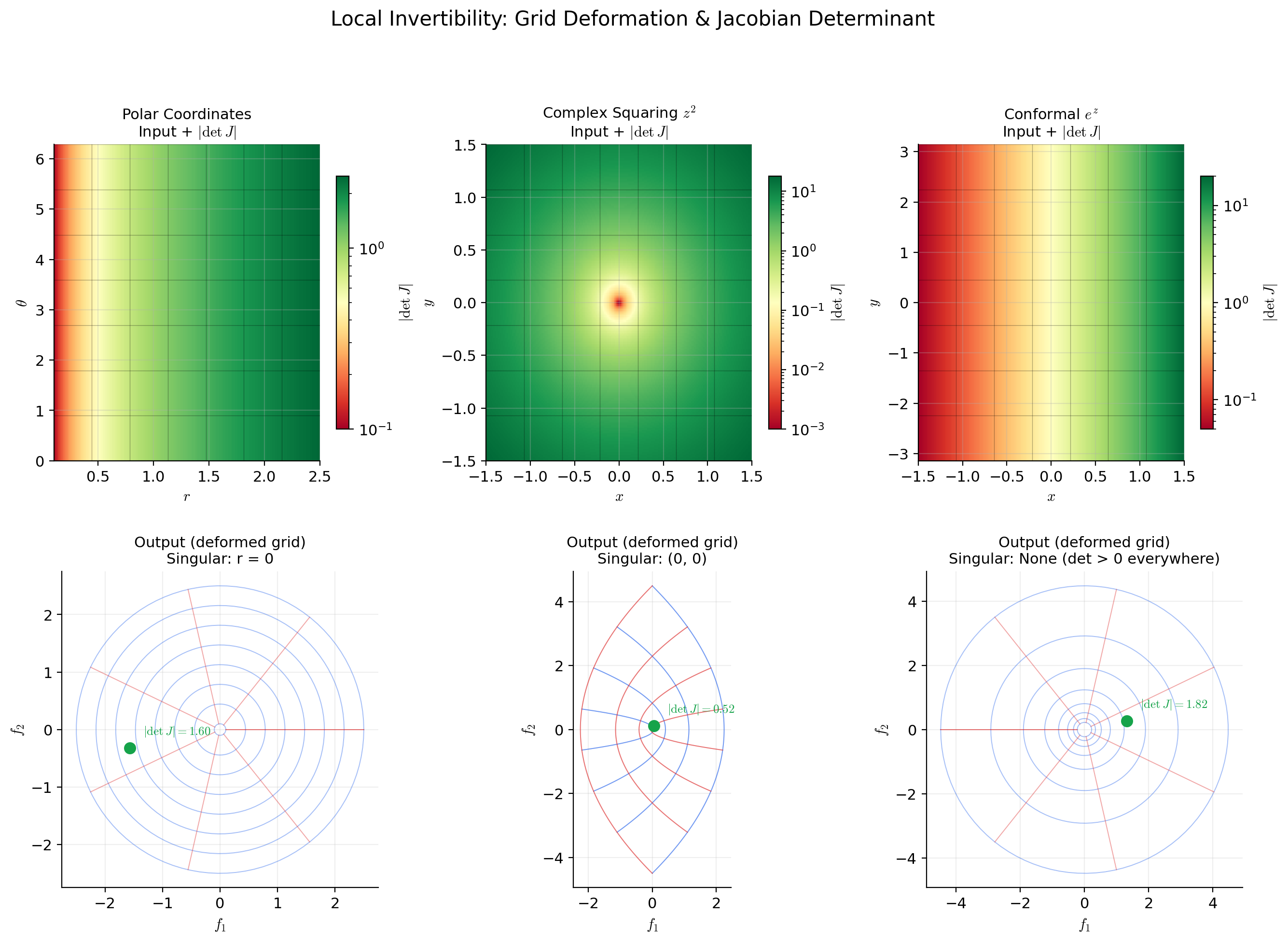
📝 Example 1 (Polar coordinates — local diffeomorphism with a singularity)
The polar coordinate map defined by
has Jacobian
with determinant . This is non-zero when , so is a local diffeomorphism everywhere except at the origin. At , the Jacobian is singular — and geometrically, all angles map to the same point . The polar coordinate map collapses an entire line (, all ) to a single point, which is the geometric source of the singularity.
Restricting to and , the map becomes a diffeomorphism onto . The restriction to is necessary to prevent and from mapping to the same point.
📝 Example 2 (Exponential map — everywhere locally invertible, not globally injective)
Define by
The Jacobian is
with everywhere. The Jacobian is never singular — the IFT guarantees that is a local diffeomorphism at every point. Yet is not globally injective: for all , because the complex exponential is -periodic. This is a clean example of the gap between “locally invertible everywhere” and “globally invertible.”
💡 Remark 1 (Local vs. global invertibility in normalizing flows)
The distinction between local and global invertibility is not merely a mathematical subtlety — it drives architectural decisions in machine learning. The IFT only guarantees local invertibility: given a non-singular Jacobian at one point, the function has a smooth inverse in some neighborhood. Normalizing flows need global bijectivity (every input maps to a unique output over the entire domain) to define valid density transformations.
Architectures like Real-NVP and NICE achieve global bijectivity by construction: affine coupling layers , are globally invertible because the triangular structure makes the inverse explicit. The IFT is not needed for these architectures — but it is needed for residual flows , where global invertibility requires additional conditions (e.g., Lipschitz constant of less than 1).
The Inverse Function Theorem
This is the central result. The hypothesis is a pointwise condition on the Jacobian; the conclusion is local invertibility with a smooth inverse.
🔷 Theorem 1 (Inverse Function Theorem (IFT))
Let be open and let be (continuously differentiable). Let and . Suppose that the Jacobian matrix is invertible (equivalently, ).
Then there exist open sets with and with such that:
- Bijection: is a bijection.
- Smooth inverse: The inverse function is .
- Derivative formula: For every ,
In words: if the linear approximation to at is invertible, then itself is invertible in a neighborhood of , with a inverse whose Jacobian is the matrix inverse of evaluated at the corresponding point.
Proof.
We prove the IFT via the Contraction Mapping Theorem (Theorem 2 below). The strategy: reformulate the equation as a fixed-point problem , show that is a contraction on a closed ball near , and invoke completeness to obtain the unique fixed point .
Setup. Let . Since , the inverse exists. Define the auxiliary map
Observe that if and only if , which (since is invertible) happens if and only if . So finding a fixed point of is equivalent to solving .
Step 1: is a contraction near . The Jacobian of with respect to is
Since is continuous (the hypothesis) and , for any there exists such that
Choose . Then for :
By the Mean Value Inequality (the multivariable Mean Value Theorem), for any :
So is a contraction with Lipschitz constant on .
Step 2: maps to itself for near . Fix (so the contraction estimate holds on ). For any :
The first term is controlled by the contraction:
For the second term:
Therefore:
This is provided . So let . For every , the map sends to itself.
Step 3: Fixed point existence and uniqueness. The closed ball is a complete metric space (closed subsets of complete metric spaces are complete, and is complete — this is where completeness enters the proof). The map is a contraction with constant .
By the Contraction Mapping Theorem (Theorem 2), has a unique fixed point . Since if and only if , we have constructed a function such that for all .
Injectivity of on : If for , then both and are fixed points of on . By uniqueness of the fixed point, . So is injective.
Surjectivity onto : For every , the fixed point satisfies , so . Therefore . (We may shrink so that .)
This establishes part (1): is a bijection with inverse .
Step 4: is . We show that is continuous, then differentiable, then .
Continuity of : For , let , so . Then:
Rearranging: . So is Lipschitz (hence continuous).
Differentiability: Since and is differentiable with invertible Jacobian (invertibility persists in a neighborhood because is a continuous function that is nonzero at , hence nonzero near ), we differentiate both sides using the chain rule:
Solving: .
regularity: The map is the composition
Each arrow is continuous: is continuous (shown above), is continuous (by the hypothesis on ), and matrix inversion is continuous on (the set of invertible matrices). Therefore is continuous, which means is .
The proof uses the Contraction Mapping Theorem as a black box. Let us now state and prove it.
🔷 Theorem 2 (Contraction Mapping Theorem (Banach Fixed-Point Theorem))
Let be a complete metric space and let be a contraction: there exists such that
Then has a unique fixed point (i.e., ). Moreover, for any starting point , the iterates converge to , with the convergence rate bound
Proof.
Existence. Pick any and define . We show is Cauchy. By the contraction property:
For , the triangle inequality gives:
Since , we have as . For any , choose such that . Then for all , . So is Cauchy.
Since is complete, the Cauchy sequence converges to some .
is a fixed point. Since is a contraction, it is Lipschitz, hence continuous. Therefore:
Uniqueness. Suppose and . Then:
Since , this implies , so , hence .
Rate bound. Letting in the estimate :
📝 Example 3 (Inverse Jacobian for the complex squaring map)
Define by — this is the real-variable form of the complex map , where .
The Jacobian is:
At : , so the IFT guarantees a local inverse near .
The inverse Jacobian is:
This tells us that a small perturbation near produces a perturbation near .
The Jacobian is singular when , i.e., at the origin — exactly where the complex squaring map has a branch point. The IFT fails at the origin, and indeed is two-to-one in every neighborhood of (except at itself).
💡 Remark 2 (Higher regularity: the C^k version)
The IFT as stated gives a inverse when is . But the regularity transfers: if is (all partial derivatives up to order exist and are continuous), then the local inverse is also . If is (smooth), so is . If is real-analytic, so is .
The key to the induction is the derivative formula . If is and is (which follows from being ), then is a composition of maps with matrix inversion, hence . But being means is .
Polar coordinates: det J = r, singular at the origin
[0.707, 1.061]
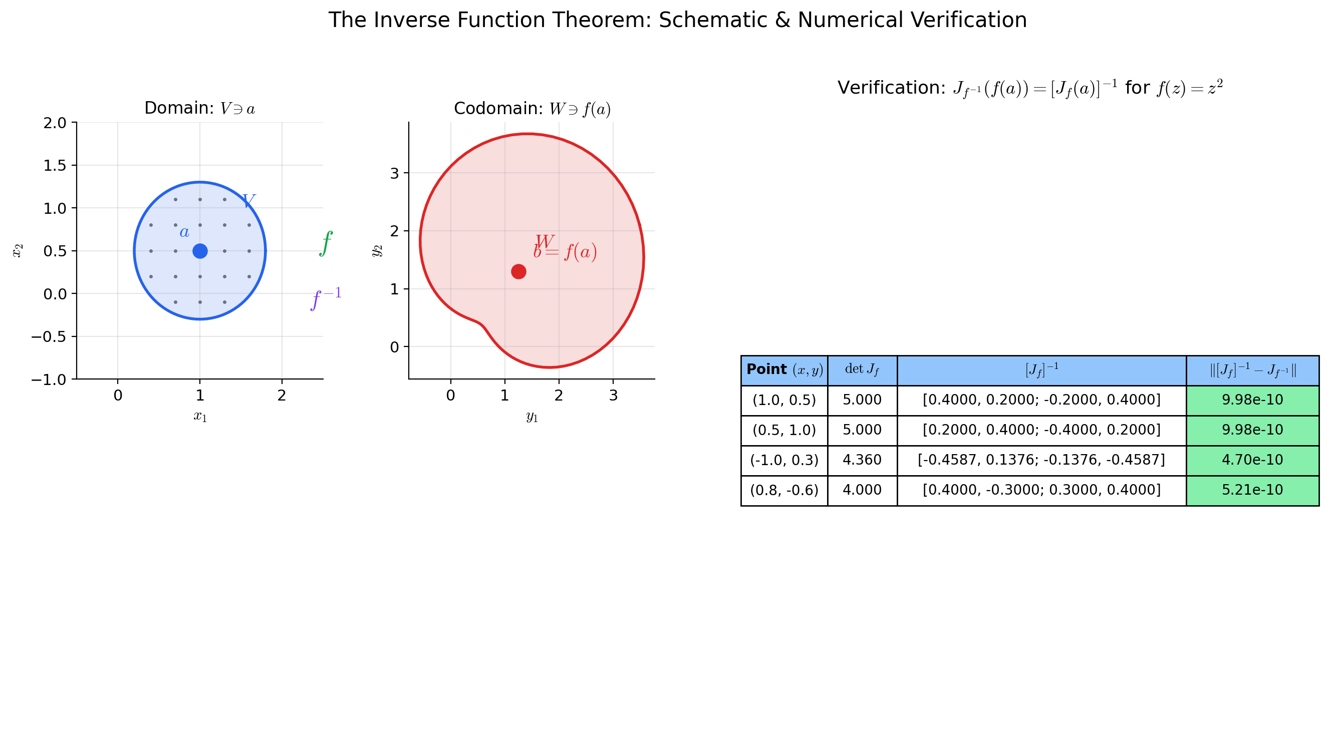
The Derivative of the Inverse
The derivative formula from the IFT proof deserves its own spotlight — it is the tool you actually use to compute derivatives of inverse functions in practice.
🔷 Proposition 1 (Jacobian of the Inverse)
Let be a diffeomorphism with inverse . Then for every :
In components: if and , then
In the scalar case , this reduces to the familiar formula .
Proof.
Differentiate with respect to using the chain rule:
Since is invertible (invertibility persists in a neighborhood of by continuity of ), multiply both sides on the left by :
📝 Example 4 (Inverse derivative for polar coordinates)
Polar coordinates: with inverse (for ).
Via the formula: At the point , so :
The determinant is . So:
Direct computation (verification):
The results agree. The formula saves us the trouble of computing the inverse function and differentiating it directly — which in higher dimensions may not be feasible.
📝 Example 5 (Inverse derivative in a normalizing flow coupling layer)
An affine coupling layer in Real-NVP splits the input and defines:
where are neural networks and is elementwise multiplication. The Jacobian is block-triangular:
The determinant is , which is always positive — so the IFT is satisfied everywhere. The inverse is explicit: . The inverse Jacobian is:
with . The entire normalizing flow density computation reduces to evaluating the network — this is why coupling layers are popular.
The Implicit Function Theorem
The Inverse Function Theorem answers “when is solvable for near a known solution?” The Implicit Function Theorem answers a more structured question: given a system where and play different roles, when can we solve for as a function of ?
📐 Definition 2 (Implicit Equation and Level Set)
Let be a map. An implicit equation is the system , where and . The level set (or solution set) is
We say is an implicit function defined by near a point if is a map defined on a neighborhood of such that for all in that neighborhood, and .
To state the theorem, we need to decompose the Jacobian of into parts corresponding to the -variables and -variables.
📐 Definition 3 (Partial Jacobians)
Let be . At a point , the partial Jacobian with respect to is the matrix
and the partial Jacobian with respect to is the matrix
The full Jacobian of viewed as a map is the block matrix .
🔷 Theorem 3 (Implicit Function Theorem (ImFT))
Let be in a neighborhood of . Suppose:
- , and
- the partial Jacobian is invertible ().
Then there exist open sets in and in such that:
- Existence and uniqueness: For every , there is a unique with .
- Smoothness: The implicit function is .
- Derivative formula:
Proof.
We derive the ImFT from the IFT by a standard augmentation trick.
Step 1: Construct an auxiliary map. Define by
So keeps unchanged and applies to get the second component. Note .
Step 2: Compute the Jacobian of . The Jacobian of at is the block matrix:
The determinant of this block-triangular matrix is:
by hypothesis. So is invertible.
Step 3: Apply the IFT to . By the Inverse Function Theorem (Theorem 1), is locally invertible near : there exist neighborhoods and and a inverse .
Since , the first component of is the identity on . Therefore the inverse has the form for some function , because the first component must invert the identity.
Step 4: Extract . Set : the equation means . Its unique solution near is . Define . Then:
- (since ),
- for all near ,
- is (as a restriction of the map ).
Step 5: Derive the derivative formula. Differentiate with respect to using the chain rule:
Solving for (using the invertibility of ):
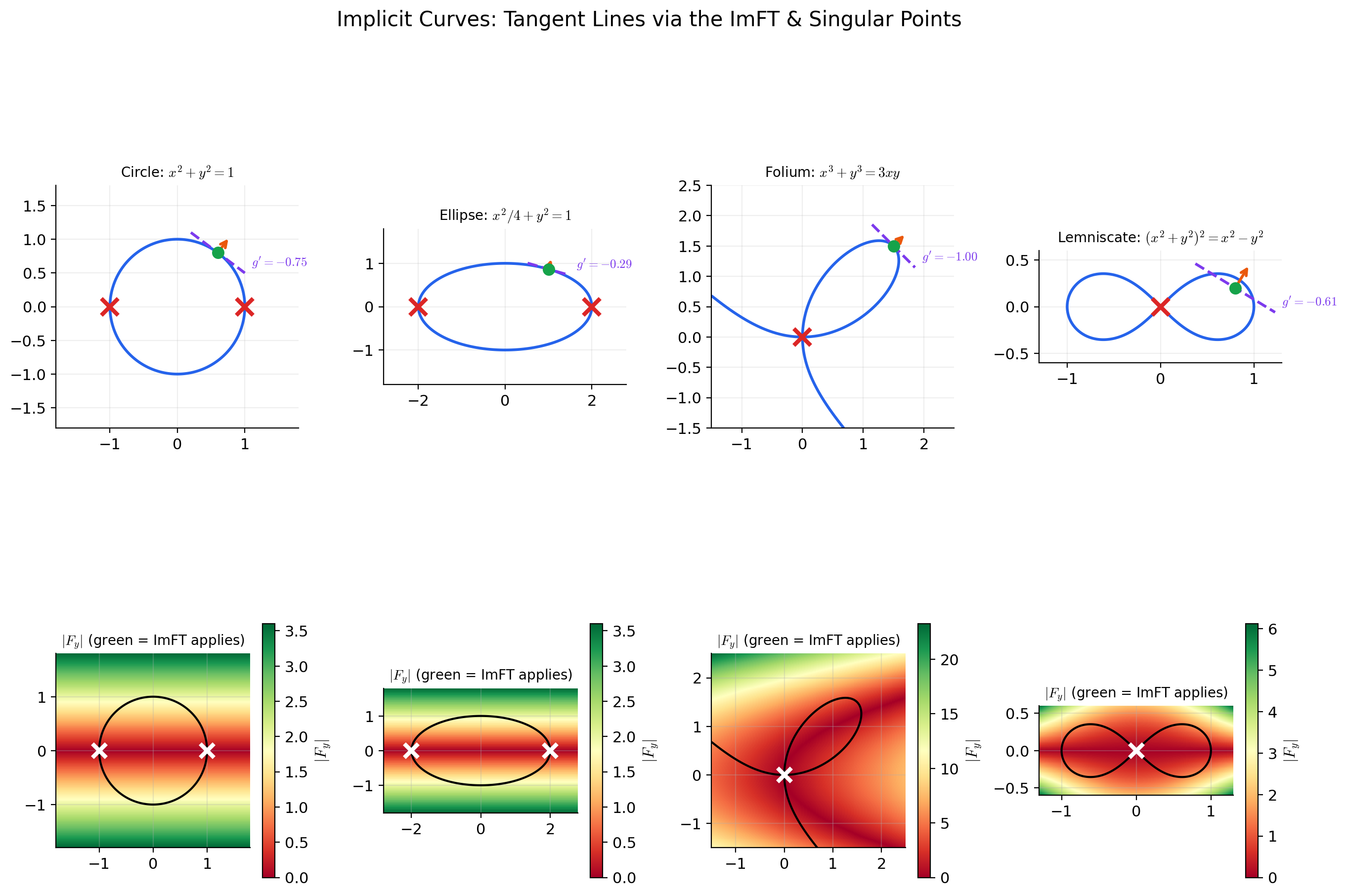
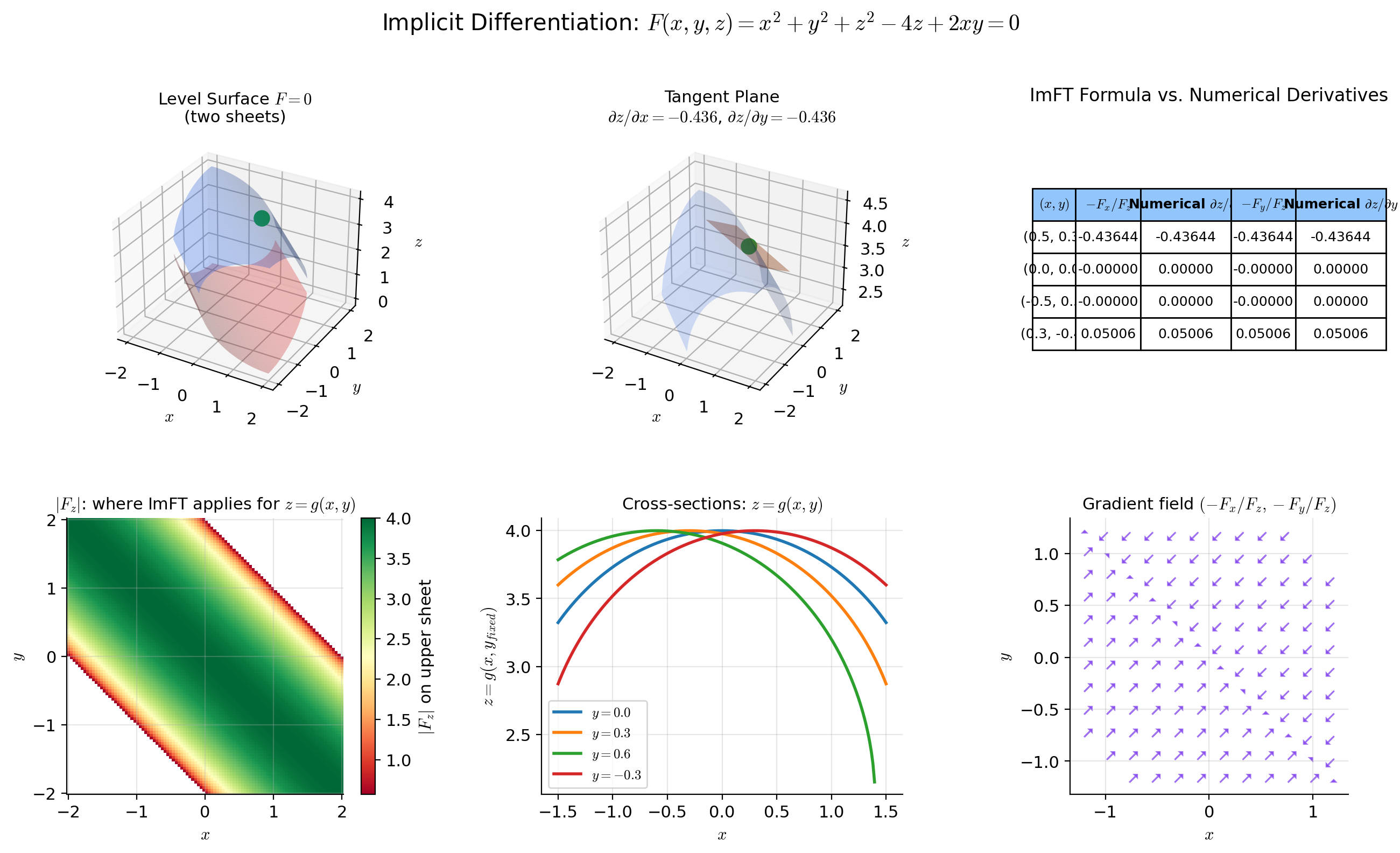
📝 Example 6 (The unit circle: x^2 + y^2 = 1)
Let . The level set is the unit circle .
We have and . The ImFT applies at any where , i.e., where .
Near : . The ImFT gives (the upper semicircle) with
Near : . The ImFT gives (the lower semicircle).
At : . The ImFT does not apply, and indeed the circle has vertical tangent lines there — cannot be expressed as a function of near these points. However, , so by applying the ImFT with the roles of and reversed, we can solve for near these points.
📝 Example 7 (A 2D system: two constraints in four variables)
Let be defined by
At the point : . Let us adjust: take . Then . Good.
The partial Jacobian with respect to :
At our point: with .
The ImFT guarantees a function with and near . The derivative is:
At our point: , so .
💡 Remark 3 (The ImFT as a corollary of the IFT)
The proof above makes the logical relationship clear: the Implicit Function Theorem is a corollary of the Inverse Function Theorem. The augmentation trick — defining to turn a rectangular system into a square one — is the standard reduction. Conversely, the IFT is a special case of the ImFT: to find such that , set and apply the ImFT. The two theorems are logically equivalent.
Unit circle: F_y = 2y = 0 at (±1, 0) — vertical tangents where the ImFT fails for y = g(x)
Implicit Differentiation
The derivative formula from the ImFT is the rigorous version of the “implicit differentiation” technique from introductory calculus. Let us spell it out and apply it.
🔷 Proposition 2 (Implicit Differentiation Formula)
Let be with and . If is the implicit function guaranteed by the ImFT, then:
In the scalar case (one equation , one unknown ):
📝 Example 8 (Implicit differentiation on the circle (verification))
. Near , the ImFT gives .
Implicit differentiation:
Direct differentiation of :
The results agree. The point of implicit differentiation is that we obtained without solving for explicitly — we only needed the partial derivatives of . In higher dimensions, where explicit solutions are typically impossible, the implicit formula is the only option.
📝 Example 9 (Tangent to an elliptic curve — singular points)
Consider the elliptic curve .
Partial derivatives: , .
Implicit derivative: .
At : (the origin is on the curve), but , so the ImFT does not apply. Also , so we can solve for as a function of near the origin. The curve passes through the origin with a vertical tangent? Let us check: near , for small . So , defined only for . The curve has a cusp-like structure near the origin.
At : and , but . Similar analysis: we can solve for but not .
At : . This point is not on the curve.
At a regular point like : . Also not on the curve. Let us find a regular point: with and . Take : , so . Then .
The singular points of an elliptic curve (where both and ) are precisely where the ImFT fails in both the -for- and -for- directions. For a non-singular elliptic curve, the gradient never vanishes on the curve, so the ImFT guarantees local graph structure everywhere on .
💡 Remark 4 (Second-order implicit differentiation)
The ImFT derivative formula gives the first derivative of . To find (which connects to the Hessian), differentiate using the quotient rule and the chain rule — remembering that depends on :
(all partials evaluated at ). This expression involves the second-order partials , , — the entries of the Hessian of . The curvature of the implicit curve is governed by the interplay between the Hessian of and the gradient of . This is the bridge between the implicit function machinery and the second-order analysis from Topic 11.
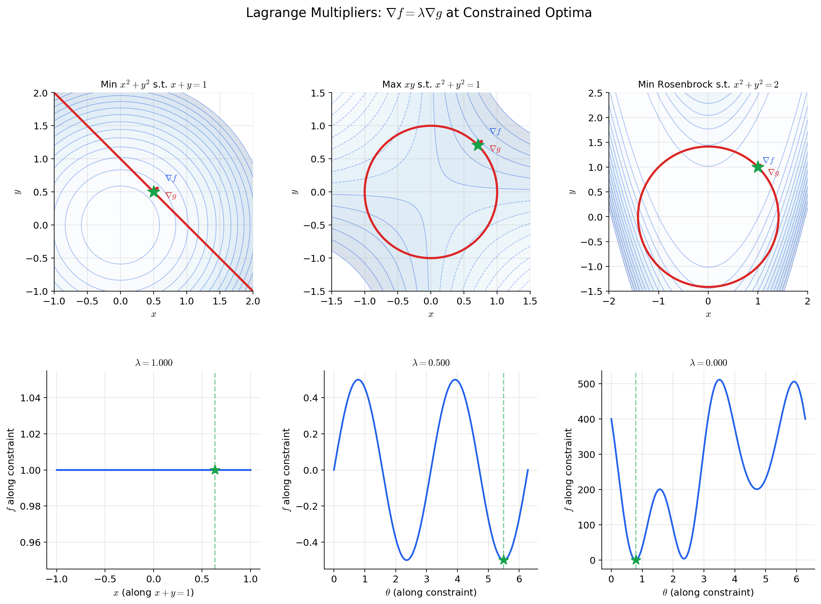
Constraint Optimization & Lagrange Multipliers
The ImFT provides the theoretical backbone for constrained optimization — the setting where we minimize a function subject to equality constraints.
📐 Definition 4 (Constrained Optimization Problem)
Given (the objective function) and with (the constraint map), the constrained optimization problem is:
The constraint set (or feasible set) is .
🔷 Theorem 4 (Lagrange Multiplier Necessary Condition)
Let and be . Suppose is a local extremum of restricted to .
Constraint qualification: If the Jacobian has full rank (equivalently, the gradients are linearly independent), then there exist unique Lagrange multipliers such that
or equivalently, where .
In the scalar constraint case (, single constraint ): .
Proof.
We use the ImFT to reduce the constrained problem to an unconstrained one.
Step 1: Apply the ImFT. Since has rank , there is an submatrix of with nonzero determinant. After reindexing, we may assume that the last columns of form an invertible matrix. Write with (the “free” variables) and (the “constrained” variables). Then
By the Implicit Function Theorem, there exists a function defined near such that . The constraint surface is locally the graph of .
Step 2: Reduce to unconstrained optimization. Define . Since is a local extremum of on , and is locally parametrized by , the point is a local extremum of on . By the standard first-order necessary condition (no constraints), , which gives:
Step 3: Use the ImFT derivative formula. From the ImFT, . Substituting:
Define , i.e., . Then:
And from the definition of :
Combining both sets of equations: .
📝 Example 10 (Maximum entropy on the probability simplex)
Maximize the entropy subject to the constraint (probabilities sum to 1). Set to convert to a minimization problem.
The Lagrange condition gives:
So for all . The constraint gives , hence for all . The uniform distribution maximizes entropy on the simplex — a foundational result in information theory.
The constraint qualification holds: , so has rank 1 everywhere.
📝 Example 11 (Nearest point on a constraint surface)
Find the point on the surface nearest to the origin. We minimize (distance squared) subject to .
Lagrange condition: .
This gives the system:
From the second equation: either or .
Case : Equation 1 gives , so . Equation 3 gives , so . Then , so . The origin satisfies but — this is the minimum, but it’s a degenerate case (the origin is on the surface).
Case : Equations 1 and 3 become and . Adding: . So . If : , giving , so . Then , requiring . If : . Then , giving again.
The geometry reveals that the only point where and is the origin — the surface passes through the origin as an isolated point (in this particular slice). The nearest nonzero point requires a more careful analysis of the full surface structure.
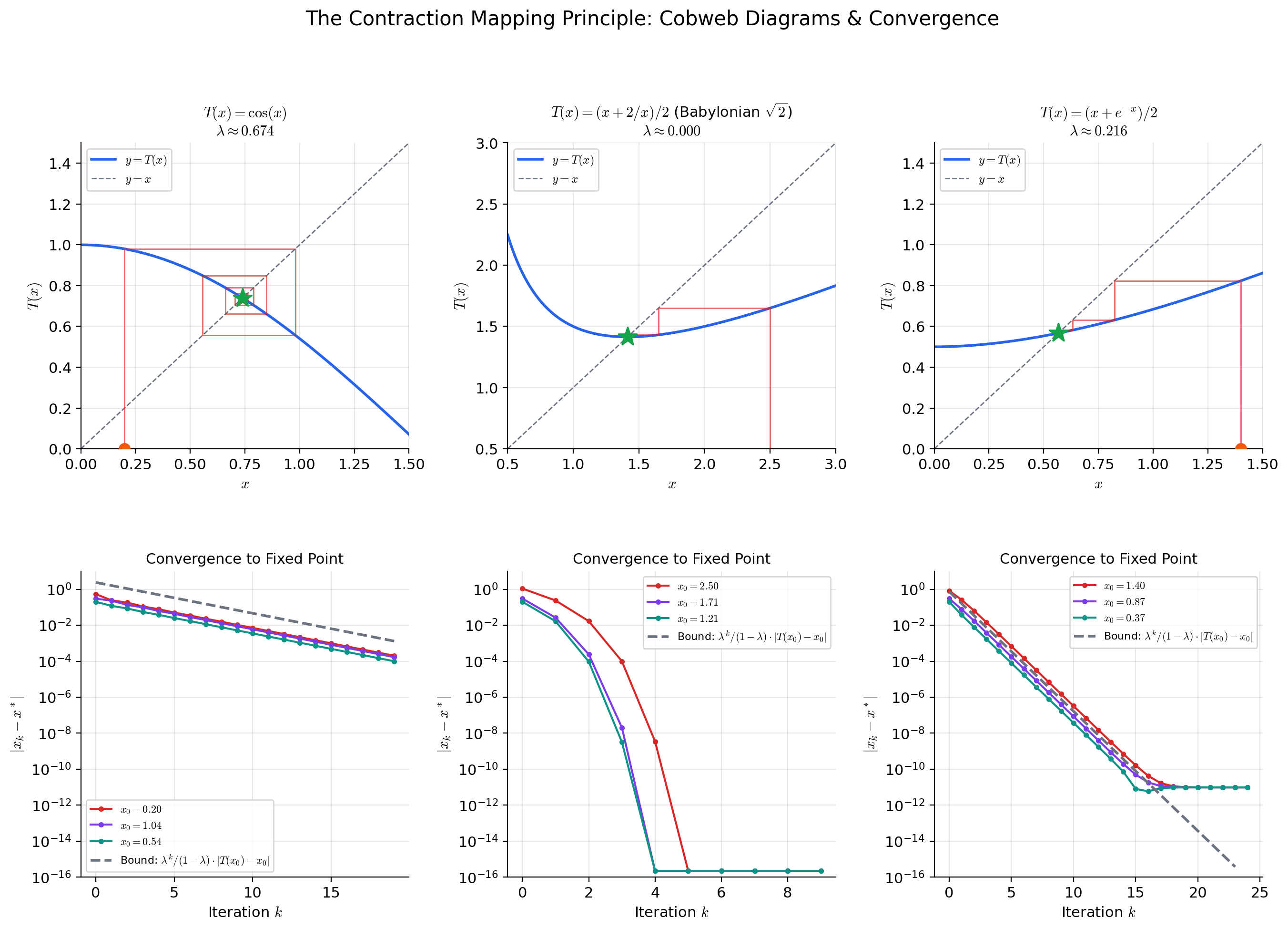
The Contraction Mapping Principle
The Contraction Mapping Theorem (Theorem 2) played a supporting role in the IFT proof, but it is a powerful tool in its own right — one of the most versatile fixed-point theorems in analysis.
📐 Definition 5 (Contraction Mapping)
Let be a metric space. A map is a contraction (or contraction mapping) if there exists a constant such that
The constant is the contraction constant (or Lipschitz constant). Every contraction is continuous (it is Lipschitz), but the crucial point is that — each application of brings points strictly closer together.
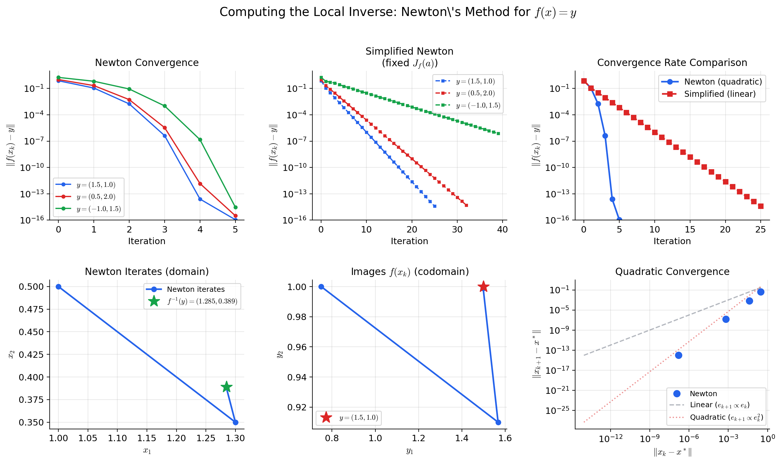
💡 Remark 5 (Newton's method as approximate contraction)
Newton’s method for solving defines the iteration . Near a root where is invertible, the Newton map satisfies (the derivative of the Newton map vanishes at the fixed point). This means is super-contractive near — the contraction constant is not merely less than 1, but tends to 0, which is why Newton’s method converges quadratically rather than geometrically.
The connection to the IFT is direct: the map used in the IFT proof is a “frozen Newton” iteration — it uses the fixed matrix instead of updating at each step. Freezing the matrix makes the analysis cleaner (the contraction constant is uniform) at the cost of slower convergence (linear instead of quadratic).
📝 Example 12 (Fixed-point iteration for x = cos(x))
The equation has a unique solution — the Dottie number. Define on .
Is a contraction? We need for all . Since on , the map is a contraction with . Also, .
Starting from : the iterates , , , , … converge (slowly) to . The rate bound gives:
After iterations: , giving about 3 digits of accuracy. Convergence is slow because is close to 1 — contrast this with the IFT proof where , which gives an extra digit of accuracy every 3-4 iterations.
Connections to Statistics
The inverse and implicit function theorems are the technical backbone of differentiating estimators and inverting tests in statistical inference.
Differentiating the MLE
The implicit function theorem justifies differentiating with respect to — needed for jackknife and influence-function calculations. The condition (non-singular Hessian at ) is exactly the identifiability condition. See formalStatistics Maximum Likelihood.
Method of moments
Solving the moment equations for is an instance of solving for . The implicit function theorem gives conditions under which the solution exists and is differentiable; its Jacobian w.r.t. drives the asymptotic variance calculation. See formalStatistics Method of Moments.
Test inversion → confidence intervals
Inverting a hypothesis test to construct a confidence interval — — is an implicit-function operation: we solve the equation “test statistic equals critical value” for as a function of . See formalStatistics Confidence Intervals & Duality.
Connections to ML
The IFT and ImFT are not abstract existence theorems that sit on the shelf — they are active structural guarantees used throughout modern machine learning. Here are three central connections.
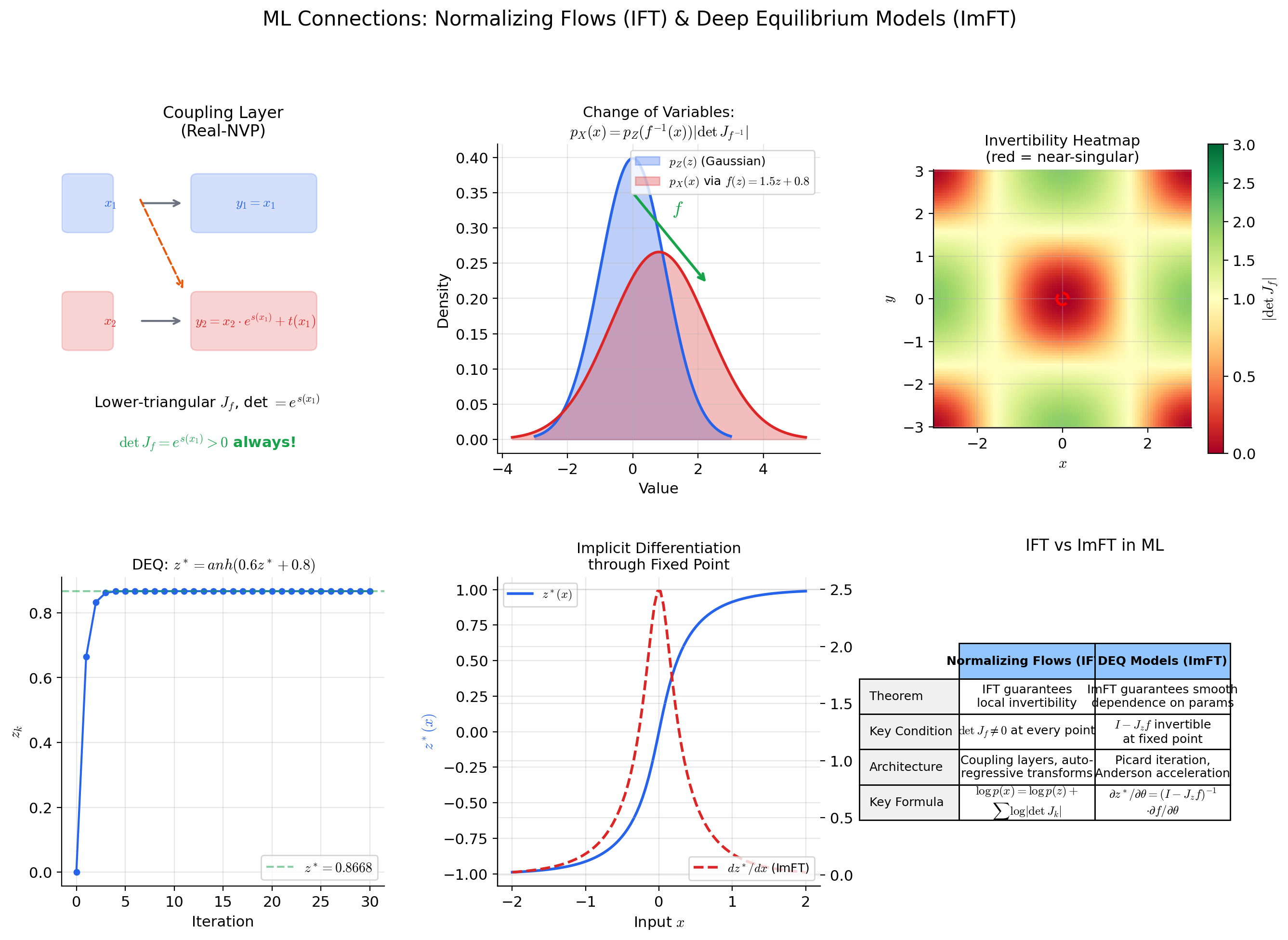
Normalizing flows and invertible neural networks
A normalizing flow transforms a simple base distribution into a complex target distribution by composing invertible layers . The change-of-variables formula gives the density:
The IFT is the theoretical guarantee behind this formula: at each layer, if , the layer is locally invertible and the density formula is valid. Architectures like Real-NVP, Glow, and Neural Spline Flows are designed so that each layer is globally invertible by construction (triangular Jacobians, monotone splines), sidestepping the “local vs. global” issue. But residual flows require the IFT: the Jacobian must be invertible at every point, which holds when (the spectral norm is less than 1) — making the map a contraction-like perturbation of the identity.
See Gradient Descent → formalML for the optimization perspective on these architectures.
Deep Equilibrium Models and implicit layers
A Deep Equilibrium Model (DEQ) defines its output implicitly: instead of stacking layers , it finds the fixed point — the “equilibrium” of the infinite-depth limit. The output is , which depends implicitly on the parameters and input .
How do we differentiate through this implicit layer? The ImFT. Define . At the fixed point, . The partial Jacobian is . If is invertible (i.e., is not an eigenvalue of ), the ImFT guarantees that varies smoothly with , and the derivative is:
This is implicit differentiation — we compute gradients through the equilibrium without backpropagating through the fixed-point iteration. The ImFT is not just a convenience here; it is the theoretical foundation guaranteeing that the gradient exists and is well-defined.
See Smooth Manifolds → formalML for the geometric perspective on implicit layers.
Constrained optimization on manifolds
Many ML problems involve optimization on constraint sets that are smooth manifolds: the Stiefel manifold (orthonormal -frames, used in spectral methods), the probability simplex (used in attention mechanisms and mixture models), and the manifold of positive definite matrices (used in covariance estimation).
The ImFT is the theorem that makes these sets manifolds in the first place. The Stiefel manifold is the level set of the map . The ImFT (via the Regular Value Theorem, Theorem 5 below) guarantees that this is a smooth manifold of dimension , with tangent spaces that can be computed from the Jacobian of .
Lagrange multipliers (Theorem 4) are then the first-order optimality conditions on these manifolds — and the entire framework of Riemannian optimization (projecting gradients onto tangent spaces, geodesic line search, retraction maps) rests on the smooth manifold structure guaranteed by the ImFT.
See Information Geometry → formalML for the Riemannian optimization perspective.
Degenerate Cases
What happens when the IFT or ImFT hypotheses fail? When , the function is not locally invertible — but the failure can be analyzed, and it leads to rich mathematical structure.
📐 Definition 6 (Critical Point of a Map)
Let be . A point is a critical point of if the Jacobian does not have full rank, i.e., . The image of a critical point is a critical value. A value that is not a critical value is a regular value — this means that for every , the Jacobian has full rank.
Note: a value is regular even if — the condition is vacuously satisfied when no preimage exists.
🔷 Theorem 5 (Regular Value Theorem)
Let be with . If is a regular value of and the level set is nonempty, then is a smooth -dimensional manifold.
More precisely: for every , there exist an open neighborhood of in and a diffeomorphism such that
The tangent space of at is , which has dimension by the rank-nullity theorem (since has rank ).
The proof follows directly from the ImFT: rewrite as . Since is regular, has rank at every point of . After reindexing variables into “free” and “constrained” groups, the ImFT provides local graph representations , which are the chart maps of the manifold structure.
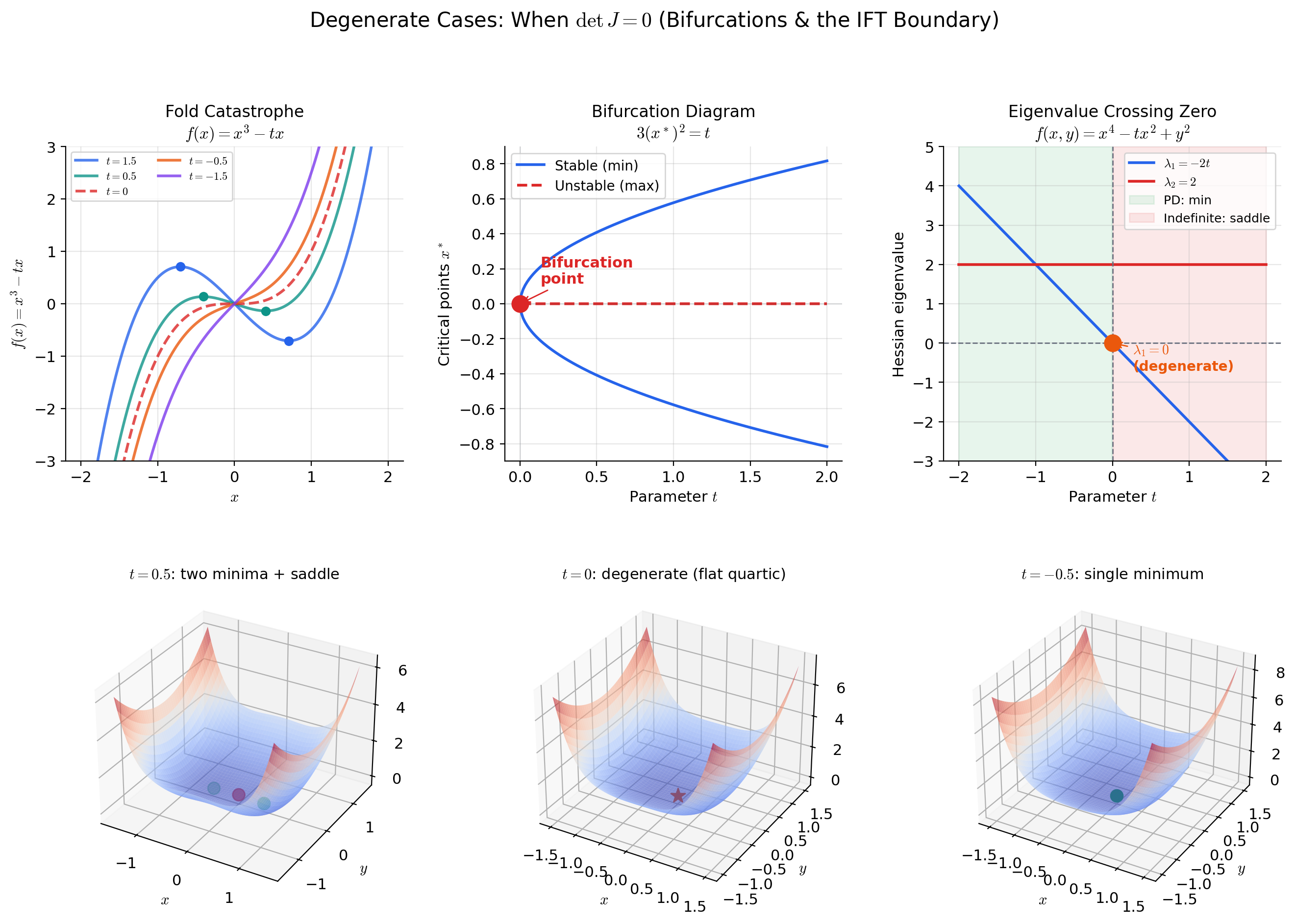
📝 Example 13 (The fold catastrophe: f(x) = x³ − tx)
Consider the family of functions parametrized by . The critical points of satisfy , giving (for ). Define the gradient map by .
The level set is the parabola — the bifurcation curve in the parameter space. On this curve, , which vanishes at . The ImFT fails at the origin: , so we cannot solve for as a smooth function of near .
This is a fold bifurcation: for , has no critical points; for , has two critical points (a local max and a local min); at , the two critical points collide and annihilate. The ImFT detects this qualitative change in structure — the smooth implicit function ceases to exist precisely at the bifurcation point.
📝 Example 14 (Loss landscape bifurcations in neural networks)
Consider a two-layer neural network with scalar weights and ReLU activation . The loss on a single data point is .
The critical points satisfy . For the ReLU network, the gradient is:
The Hessian — the Jacobian of the gradient — is singular whenever the ReLU transitions between active and inactive: at , the function is not differentiable, and the smooth landscape splits into two regions. This is a form of bifurcation in the loss landscape: the topology of the critical point set changes as crosses zero. The IFT applied to the gradient map tells us that critical points are isolated (and vary smoothly with hyperparameters) wherever is non-singular — exactly the Hessian condition from Topic 11.
💡 Remark 6 (The rank theorem and the road to differential topology)
The IFT and ImFT are the starting points of differential topology — the study of smooth manifolds and smooth maps between them. The Regular Value Theorem (Theorem 5) is the bridge: it tells us that level sets of smooth maps are generically manifolds. The rank theorem generalizes this: near a point where has constant rank , the map can be locally reduced (by smooth coordinate changes in both domain and range) to the linear projection . Maps of constant rank are submersions (when , the map is “onto” locally) and immersions (when , the map is “one-to-one” locally). The IFT is the special case where .
For the connection to manifold theory in the ML context, see Smooth Manifolds → formalML.
Computational Notes
The IFT and ImFT tell us when inverse and implicit functions exist; computation requires numerical methods. Here are the essential tools.
Solving implicit equations: scipy.optimize.fsolve
import numpy as np
from scipy.optimize import fsolve

# Find y such that F(x, y) = x^2 + y^2 - 1 = 0, near y = 0.8
def F(y, x):
    return x**2 + y**2 - 1

x_val = 0.5
y_solution = fsolve(F, x0=0.8, args=(x_val,))
print(f"y = {y_solution[0]:.6f}")  # y ≈ 0.866025 = sqrt(3)/2
Computing inverse Jacobians: np.linalg.solve vs. np.linalg.inv
import numpy as np

# Jacobian of the complex squaring map at (1, 1)
J_f = np.array([[2, -2],
                [2,  2]])

# Bad: explicit inverse (O(n^3), numerically unstable for large n)
J_g_bad = np.linalg.inv(J_f)

# Good: solve J_f @ J_g = I directly (same cost, better stability)
J_g_good = np.linalg.solve(J_f, np.eye(2))

print("Inverse Jacobian:\n", J_g_good)
print("Condition number:", np.linalg.cond(J_f))
Implicit differentiation with JAX: jax.custom_vjp
import jax
import jax.numpy as jnp
from functools import partial

def fixed_point_layer(params, x, f, max_iter=100, tol=1e-6):
    """Find z* such that z* = f(params, x, z*)."""
    z = jnp.zeros_like(x)
    for _ in range(max_iter):
        z_new = f(params, x, z)
        if jnp.max(jnp.abs(z_new - z)) < tol:
            break
        z = z_new
    return z

@jax.custom_vjp
def deq_layer(params, x):
    f = lambda p, x, z: jnp.tanh(p @ z + x)  # Example implicit layer
    return fixed_point_layer(params, x, f)

def deq_layer_fwd(params, x):
    z_star = deq_layer(params, x)
    return z_star, (params, x, z_star)

def deq_layer_bwd(res, g):
    """Backward pass via ImFT: dz*/dtheta = (I - df/dz)^{-1} df/dtheta."""
    params, x, z_star = res
    # Solve (I - J_f) @ v = g for v, where J_f = df/dz at z*
    f = lambda z: jnp.tanh(params @ z + x)
    J_f = jax.jacobian(f)(z_star)
    v = jnp.linalg.solve(jnp.eye(len(z_star)) - J_f, g)
    # Propagate through df/dparams and df/dx
    params_grad = jnp.outer(v, jnp.where(1 - jnp.tanh(params @ z_star + x)**2 > 0,
                                          z_star, 0))
    x_grad = v * (1 - jnp.tanh(params @ z_star + x)**2)
    return params_grad, x_grad

deq_layer.defvjp(deq_layer_fwd, deq_layer_bwd)
Constrained optimization with SciPy
from scipy.optimize import minimize

# Maximize entropy on the simplex (n=3)
def neg_entropy(p):
    return np.sum(p * np.log(p + 1e-12))

def constraint_sum(p):
    return np.sum(p) - 1.0

result = minimize(neg_entropy, x0=[0.2, 0.3, 0.5],
                  constraints={'type': 'eq', 'fun': constraint_sum},
                  bounds=[(1e-10, 1)] * 3)
print(f"Optimal p: {result.x}")  # Should be ≈ [1/3, 1/3, 1/3]
💡 Remark 7 (Numerical vs. mathematical invertibility — the condition number)
The IFT says that is locally invertible when . Numerically, the question is how far from zero the determinant is — or more precisely, how well-conditioned the Jacobian is. The condition number (where are the singular values) measures the sensitivity of the inverse to perturbations.
If and you are working in double precision (about 16 digits), the inverse is computed with roughly zero digits of accuracy. The map is mathematically invertible but numerically singular. In normalizing flows, this manifests as numerical overflow in computations — the density estimate blows up. Architectures like Real-NVP avoid this by ensuring triangular Jacobians with bounded diagonal entries.
The rule: never compute explicitly. Instead, solve using np.linalg.solve (LU decomposition) or iterative methods. This is more numerically stable and often faster.
Connections & Further Reading
Prerequisites — topics you need first
The Jacobian & Multivariate Chain Rule
The Jacobian matrix J_f(a) is the central object of both theorems. The IFT hypothesis det J_f(a) ≠ 0 says the linear approximation is invertible; the conclusion is that the nonlinear function itself is locally invertible. The chain rule J_{f⁻¹}(f(a)) · J_f(a) = I gives the derivative of the inverse.
The Hessian & Second-Order Analysis
The Hessian H_f(a) = J(∇f)(a) is the Jacobian of the gradient map. Non-singularity of the Hessian at a critical point — the condition that makes the second derivative test conclusive — is exactly the IFT condition applied to ∇f: the gradient map is locally invertible, so the critical point is isolated.
Partial Derivatives & the Gradient
For scalar-valued functions f: ℝⁿ → ℝ, the gradient ∇f is the constraint surface normal. The Implicit Function Theorem applied to the level set f(x) = c recovers the geometry of gradient orthogonality to contours developed in Topic 9.
Completeness & Compactness
The contraction mapping proof of the IFT uses completeness of ℝⁿ as a metric space: Cauchy sequences converge, so the iterative scheme converges to a fixed point. This is the first time completeness is used in a multivariable context — connecting Track 1 foundations to Track 3 existence theorems.
Epsilon-Delta & Continuity
The IFT is an existence theorem — its proof requires careful ε-δ arguments to control the size of neighborhoods where invertibility holds. The continuity of J_f (the C¹ hypothesis) is essential: it ensures that the Jacobian stays invertible in a neighborhood, not just at a single point.
Where this leads — next in formalCalculus
On to formalStatistics — where this calculus powers inference
Maximum Likelihood
The implicit function theorem justifies differentiating θ̂(x) with respect to x (needed for Jackknife and influence-function calculations). The condition — non-singular Hessian at θ_0 — is exactly the identifiability condition.
Method Of Moments
Solving the moment equations E_θ[g(X)] = n⁻¹ Σ g(X_i) for θ is an instance of solving F(θ, x̄) = 0 for θ. The implicit function theorem gives conditions under which the solution θ̂(x̄) exists and is differentiable; its Jacobian w.r.t. x̄ drives the asymptotic variance.
Confidence Intervals And Duality
Inverting a hypothesis test to construct a confidence interval — CI(x) = {θ : test does not reject at x} — is an implicit-function operation: we solve the equation 'test statistic equals critical value' for θ as a function of x.
On to formalML — where this calculus powers ML
Gradient Descent
The IFT guarantees local convergence of gradient descent near non-degenerate minima: the gradient map is locally invertible when the Hessian is non-singular, ensuring that small perturbations from the optimum produce proportional gradient signals.
Smooth Manifolds
The Implicit Function Theorem is the foundational tool for proving that level sets are smooth manifolds. The regular value theorem — that F⁻¹(c) is a manifold when J_F has full rank on the level set — is a direct consequence of the ImFT.
Information Geometry
The statistical manifold of a parametric family is locally diffeomorphic to ℝⁿ via the IFT when the Fisher information matrix is non-singular. Reparametrization invariance relies on the IFT to guarantee that coordinate changes on the parameter space are locally invertible.
Causal Inference Methods
§9's instrumental-variables identification argument relies on the implicit-function theorem to ensure the first-stage map $e(Z) \to D$ is locally invertible when the relevance condition $\operatorname{Cov}(Z, D) \neq 0$ holds. The rank condition for IV identification is an inverse/implicit-function existence claim at the population level.
Normalizing Flows
The inverse-function theorem underpins the local-invertibility argument that justifies parameterizing flows by their forward direction: if $\det \partial T/\partial z > 0$ everywhere, $T$ is locally a diffeomorphism with smooth inverse, and the algebraic invertibility of the layer parameterization (§4.5) extends this to global invertibility.
Meta Learning
Implicit MAML (Rajeswaran et al. 2019) bypasses recursive autograd by inverting the inner-loop fixed point via the implicit function theorem. The §3.5 meta-gradient computation — equation (3.8) — is a direct application of the inverse-and-implicit calculus developed here.
Riemann Manifold Hmc
RMHMC's generalized leapfrog integrator has implicit momentum and position updates whose well-posedness (existence and uniqueness of the fixed point at small step size) is a direct IFT application: at ε = 0 the map is the identity, and the IFT extends invertibility to a neighborhood of ε = 0.
References
- book Munkres (1991). Analysis on Manifolds Chapter 7 develops the Inverse Function Theorem and the Implicit Function Theorem with careful attention to the neighborhoods where invertibility holds — the primary reference for our treatment
- book Spivak (1965). Calculus on Manifolds Chapter 2 proves the IFT via contraction mapping and derives the ImFT as a corollary — the cleanest modern treatment and our model for the proof structure
- book Rudin (1976). Principles of Mathematical Analysis Chapter 9, Theorems 9.24 and 9.28 — the IFT and ImFT in Rudin's characteristically concise style. Useful for the contraction mapping setup
- book Lee (2013). Introduction to Smooth Manifolds Chapter 4 uses the IFT/ImFT to define submersions, immersions, and the regular value theorem — the direct bridge to the smooth manifolds topic on formalml.com
- book Nocedal & Wright (2006). Numerical Optimization Chapter 12 on constrained optimization via Lagrange multipliers — the practical application of the ImFT in optimization
- paper Chen, Rubanova, Bettencourt & Duvenaud (2018). “Neural Ordinary Differential Equations” Neural ODEs use the IFT implicitly: the flow map of an ODE is locally invertible when the vector field is smooth, and the adjoint method computes gradients through this inverse
- paper Dinh, Sohl-Dickstein & Bengio (2017). “Density Estimation using Real-NVP” Normalizing flows construct diffeomorphisms with tractable Jacobian determinants — the IFT guarantees invertibility at every point in the flow
- paper Bai, Kolter & Koltun (2019). “Deep Equilibrium Models” DEQs find fixed points of implicit layers and differentiate through them via the ImFT — the canonical ML application of implicit differentiation