The Jacobian & Multivariate Chain Rule
Derivatives of vector-valued functions as matrices — the Jacobian as the best linear approximation, the chain rule as matrix multiplication, and the determinant as volume scaling
Abstract. The Jacobian matrix extends differentiation from scalar-valued functions f: ℝⁿ → ℝ to vector-valued functions f: ℝⁿ → ℝᵐ. Where the gradient is a single row of partial derivatives (the derivative of a function with one output), the Jacobian stacks m such rows — one for each output component. The Jacobian J_f(a) is the matrix representation of the total derivative Df(a): ℝⁿ → ℝᵐ, the best linear approximation to f near a. The central result is the multivariate chain rule: if g: ℝⁿ → ℝᵏ and f: ℝᵏ → ℝᵐ are differentiable, then the Jacobian of the composition f ∘ g is the matrix product J_{f∘g}(a) = J_f(g(a)) · J_g(a). This is the chain rule from single-variable calculus (multiply the derivatives along the chain) generalized to arbitrary dimensions — and it is exactly backpropagation. Every layer in a neural network computes a function fₖ: ℝⁿₖ → ℝⁿₖ₊₁, and the end-to-end Jacobian is the product J_L · J_fₖ · ⋯ · J_f₁. Reverse-mode automatic differentiation (backprop) computes this product right-to-left, one vector-Jacobian product at a time, at a cost independent of the number of parameters, which is why deep learning works at scale. For square Jacobians (n = m), the Jacobian determinant det J_f(a) measures how f distorts local volumes: areas near a are scaled by |det J_f(a)|, and the sign encodes orientation. This appears in the change-of-variables formula for integration (the r in r dr dθ for polar coordinates is the Jacobian determinant) and in normalizing flows, where the density of a transformed variable requires dividing by |det J_f|.
Overview & Motivation
In the previous topic, we differentiated functions — one output. The gradient told us how that single output changes in every input direction. But a neural network layer is not a scalar-valued function. A layer takes a vector of activations and produces a vector of activations — multiple inputs, multiple outputs. To differentiate such a function, we need a partial derivative for every input-output pair: how does the -th output change when the -th input is nudged?
Arranging all of these into a matrix gives the Jacobian. And the chain rule — the engine that makes backpropagation possible — says that the Jacobian of a composition is the product of the Jacobian matrices. If that sounds like matrix multiplication, it is. The single-variable chain rule from Topic 5 was multiplying matrices. Now we see the general picture.
This topic develops three ideas: the Jacobian matrix (the derivative of a vector-valued function), the multivariate chain rule (matrix multiplication along a computation graph), and the Jacobian determinant (how a differentiable map distorts volumes). Together, these are the calculus that makes deep learning — and much of mathematical physics — work.
Vector-Valued Functions & the Jacobian Matrix
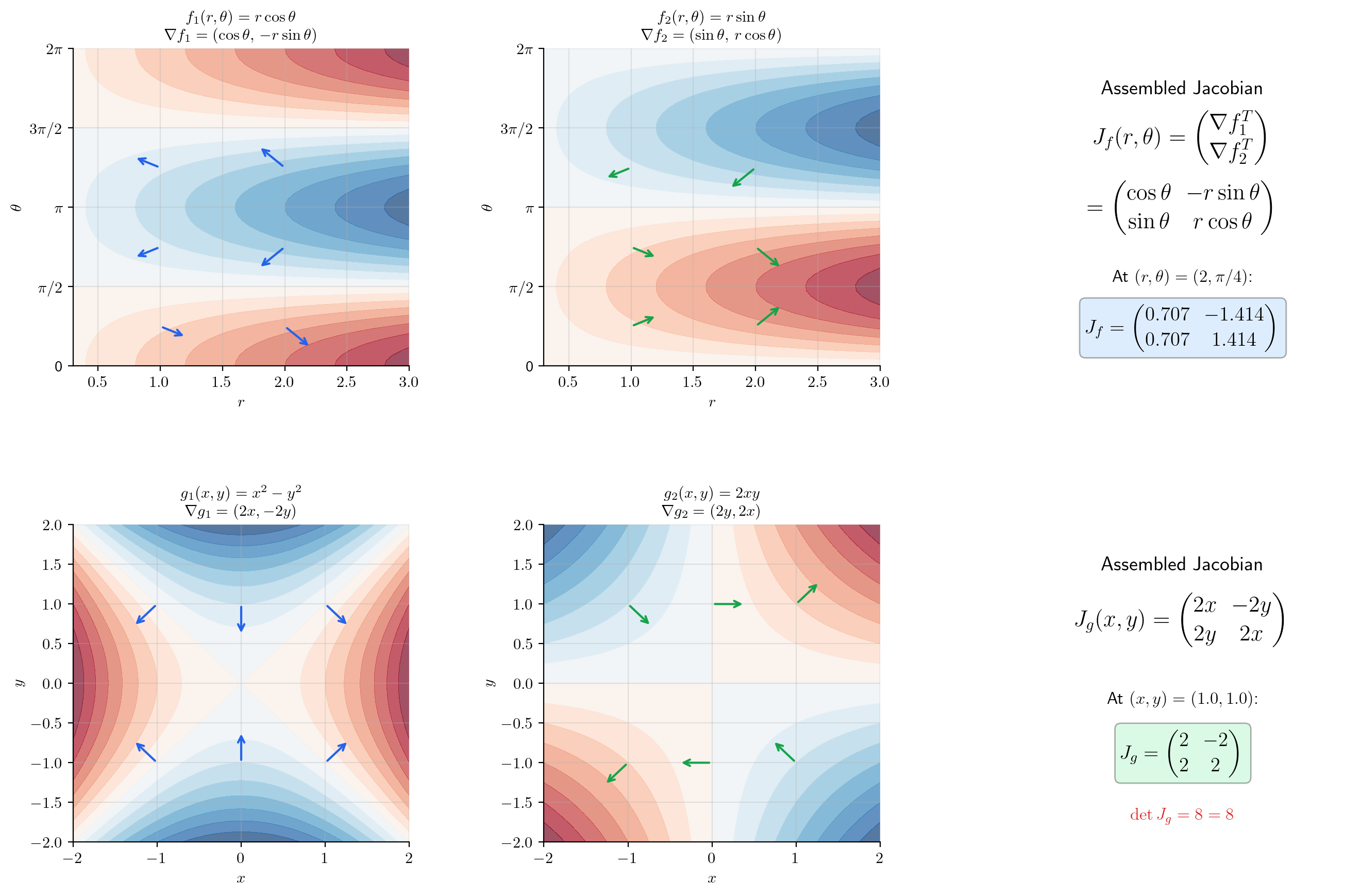
We begin with the conceptual step from scalar to vector. A function maps a region in the plane to another region in the plane. Each output component is a scalar-valued function of two variables, and each has its own gradient. The Jacobian stacks these gradients as rows.
📐 Definition 1 (Vector-Valued Function)
A vector-valued function is defined by component functions , where each is a scalar-valued function. The function maps a point to the vector
When , this reduces to the scalar-valued functions of Topic 9.
📐 Definition 2 (The Jacobian Matrix)
Let and suppose all partial derivatives exist. The Jacobian matrix (or simply Jacobian) of at is the matrix
Row of is — the gradient of the -th component function. Column is the vector of all partial derivatives with respect to . Common notations include , , and .
📝 Example 1 (Jacobian of a linear function)
Let where is a constant matrix. Then for all — the Jacobian of a linear function is the matrix itself. The derivative of a linear map is the linear map. This is the multivariable analog of ” has derivative .”
📝 Example 2 (Jacobian of polar-to-Cartesian)
Let . The Jacobian is
At , we get . The first column tells us how changes when we increase (move radially outward); the second column tells us how changes when we increase (move tangentially).
📝 Example 3 (Jacobian of a neural network layer)
A fully connected layer with activation is where is applied component-wise. By the chain rule (which we will prove shortly),
When is the identity (linear layer), — recovering Example 1. When , the diagonal matrix of values modulates each row of : the partial derivative is , where is the pre-activation vector.
💡 Remark 1 (Gradient as a special case)
When , the Jacobian is a row matrix: . The gradient is the transpose of the single-row Jacobian. When , the Jacobian is an column matrix — just the vector of ordinary derivatives of each component. When , the Jacobian is a matrix containing the single-variable derivative from Topic 5. The Jacobian unifies all of these cases.
[0.707, 1.414]
The Jacobian as Linear Approximation
Just as the gradient was the best linear approximation for (Topic 9, §7), the Jacobian is the best linear approximation for . The total derivative is a linear map , and its matrix representation is the Jacobian.
📐 Definition 3 (Differentiability (Vector-Valued))
A function is differentiable at if there exists a linear map such that
When exists, it is unique and represented by the Jacobian matrix: for all . This extends Definition 4 of Topic 9 from to arbitrary .
🔷 Theorem 1 (Differentiability ⟺ Component-wise Differentiability)
is differentiable at if and only if each component is differentiable at (in the sense of the total derivative from Topic 9). When is differentiable, the rows of the Jacobian are the gradients of the component functions.
Proof.
() If is differentiable at , then . For each component , the absolute value of a single component is bounded by the norm of the full vector:
So each is differentiable at with total derivative .
() If each is differentiable at , then for each : . We square and sum over all components:
Each summand is by hypothesis, so the sum is . Taking the square root: .
🔷 Proposition 1 (The Jacobian Approximation)
If is differentiable at , then
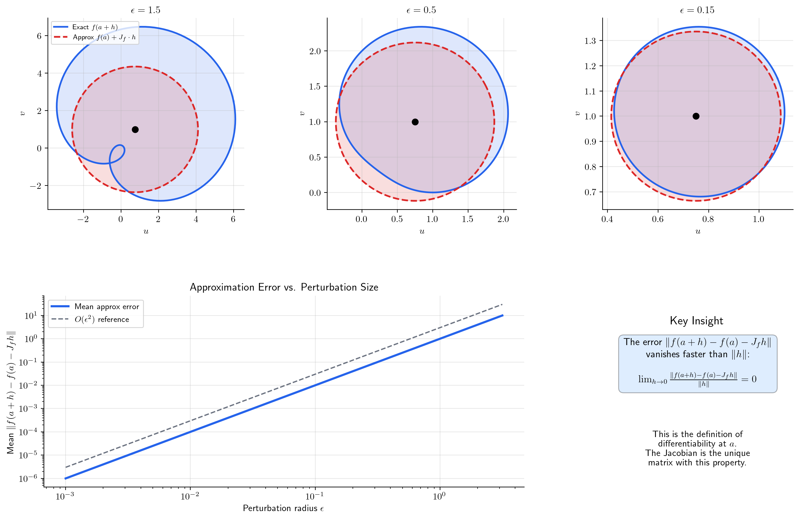
with error . This is the multivariable Taylor expansion to first order for vector-valued functions. Geometrically: the affine map is the best linear approximation to near .
📝 Example 4 (Linear approximation of polar-to-Cartesian)
Near , the polar-to-Cartesian map is approximated by
A small change in maps to a change in via matrix multiplication — the Jacobian acts on the perturbation vector. The interactive visualization below lets you see how the linear approximation (an ellipse) converges to the true image (a deformed curve) as the perturbation shrinks.
The Multivariate Chain Rule
This is the central result of the topic. The chain rule says: the derivative of a composition is the product of the derivatives. In single-variable calculus (Topic 5), this meant multiplying numbers: . Now, the “derivatives” are matrices, and the “product” is matrix multiplication.
🔷 Theorem 2 (The Multivariate Chain Rule)
Let be differentiable at , and let be differentiable at . Then the composition is differentiable at , and
The Jacobian of the composition is the matrix product of the Jacobians, evaluated at the appropriate points. The dimensions are consistent: is , is , so is — matching the expected size for a function from to .
Proof.
This is the most important proof in this topic. We track the error terms through two layers of the total derivative.
By differentiability of at , we can write
where as (here is a vector in ). By differentiability of at , we can write
where as . Set . Then
Substituting the expression for :
First error term: . The operator norm is a fixed constant, and as , so this entire term is .
Second error term: We need . From the definition: . For sufficiently small, , so for a constant . As , we have , so . Therefore .
Combining both error terms, we have shown
which proves that is differentiable at with .
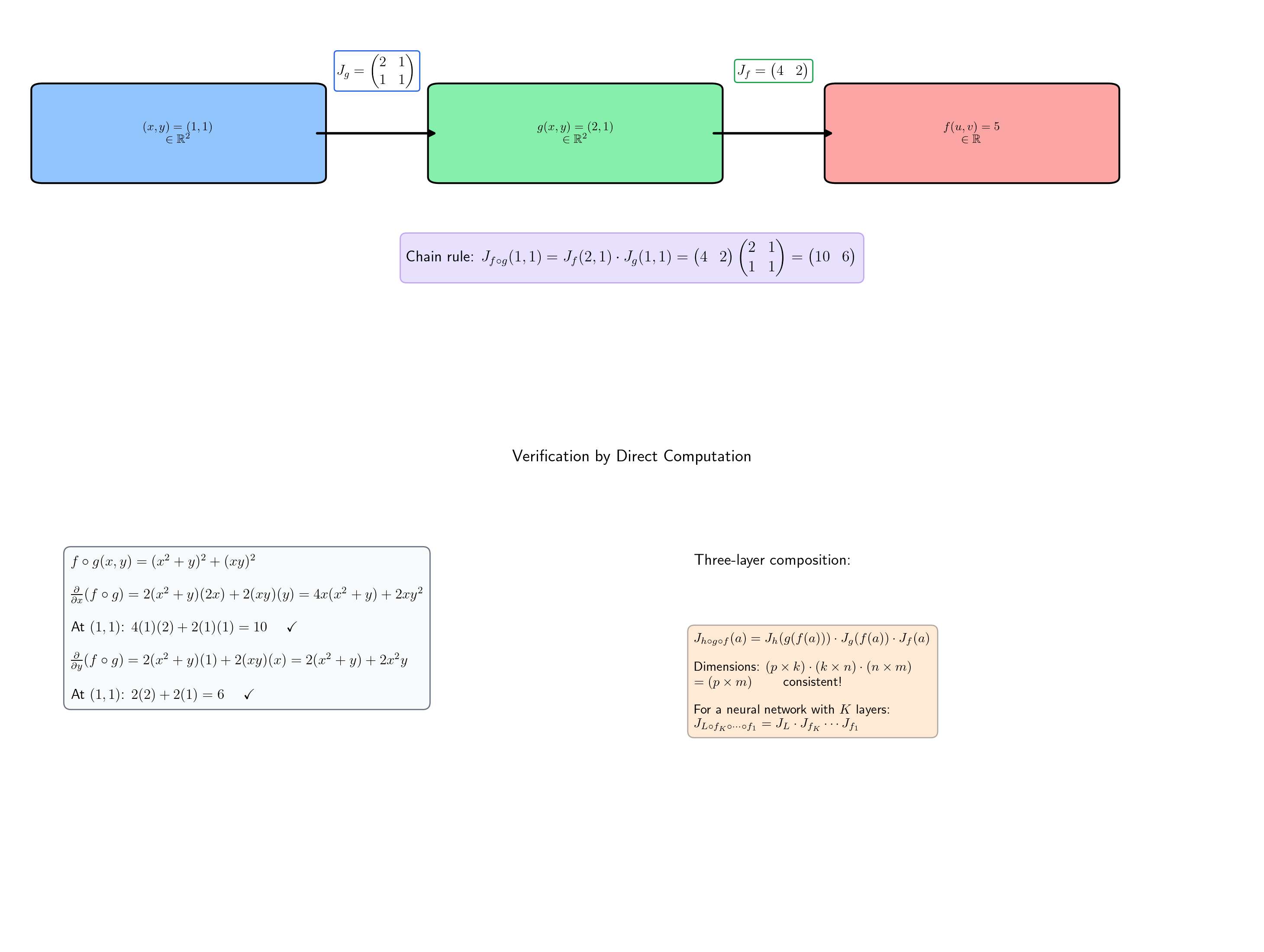
📝 Example 5 (Chain rule with explicit matrices)
Let by and by . Their Jacobians are
At : , so and .
Chain rule:
Verification by direct computation: . Then . At : . Confirmed.
📝 Example 6 (Three-fold composition)
For a three-layer chain :
The chain rule applies recursively — each Jacobian is evaluated at the appropriate intermediate value. This is the prototype for backpropagation through layers: the end-to-end Jacobian is , with each factor evaluated at the activation from the forward pass.
💡 Remark 2 (Why matrix multiplication?)
The chain rule is matrix multiplication because derivatives are linear maps, and composition of linear maps corresponds to matrix multiplication. The single-variable chain rule multiplies matrices — it just happens to look like scalar multiplication. In , the matrix structure is exposed, and the product captures how sensitivities propagate through layers of computation.
The Jacobian Determinant
When (square Jacobian), the determinant has a geometric meaning: it measures how scales volumes near .
📐 Definition 4 (The Jacobian Determinant)
For with all partial derivatives existing at , the Jacobian determinant is
The Jacobian determinant is defined only when the Jacobian is square ().
🔷 Theorem 3 (Volume Distortion)
Let be continuously differentiable near , and let be a small rectangular region containing . Then the image has volume approximately
as the diameter of shrinks to zero. The absolute value handles orientation: means preserves orientation; means it reverses orientation (like a reflection).
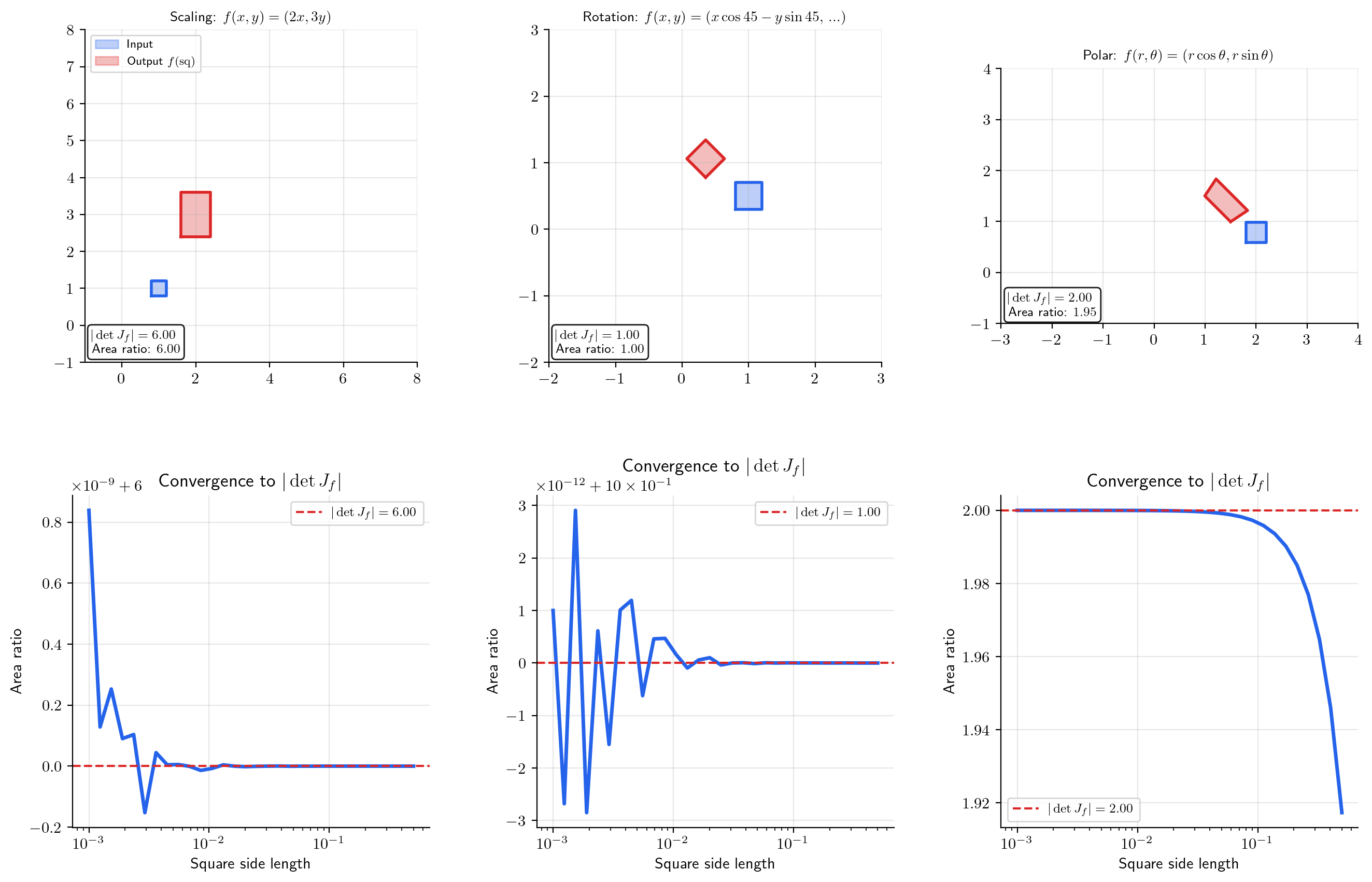
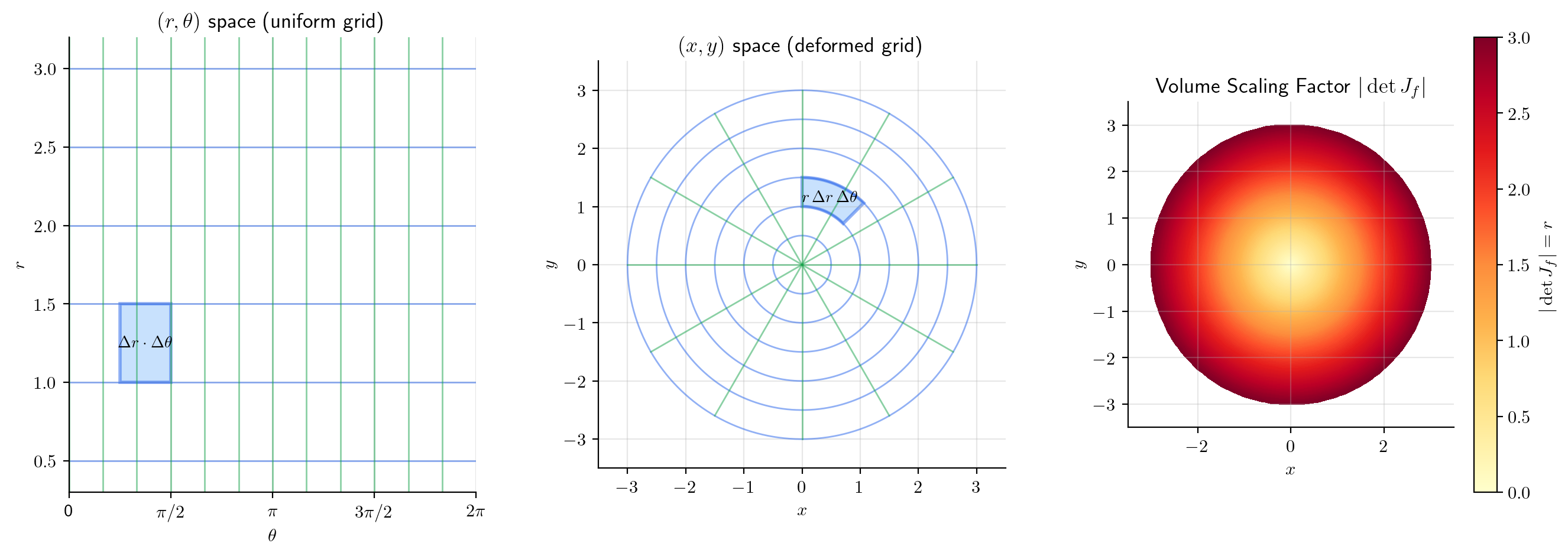
📝 Example 7 (Polar coordinates)
For :
This is the in "" for polar integration. A small rectangle in polar coordinates maps to a region of area approximately in Cartesian coordinates. Far from the origin ( large), the same angular increment covers more Cartesian area; near the origin ( small), less.
📝 Example 8 (Scaling transformation)
For : , . Every region’s area is multiplied by 6 — stretching by 2 in and by 3 in scales areas by . The determinant of a diagonal matrix is the product of the diagonal entries, and each entry is a stretch factor along one axis.
🔷 Proposition 2 (Jacobian Determinant of a Composition)
For ,
Proof.
This follows from the chain rule (Theorem 2) and the multiplicativity of determinants:
Geometrically: volume distortions compose multiplicatively. If scales volume by factor 3 and scales volume by factor 2, then scales volume by factor 6.
💡 Remark 3 (When the Jacobian determinant is zero)
means the linear approximation is not invertible — it “collapses” a neighborhood of into a lower-dimensional set. This is the boundary between the Inverse Function Theorem applying (nonzero determinant implies is locally invertible) and failing (zero determinant implies a critical value). Inverse & Implicit Function Theorems develops this connection.
Coordinate Transformations
Coordinate transformations are the most concrete application of the Jacobian determinant. We have already seen polar coordinates (Example 7). Here we systematize the pattern.
Polar coordinates: , with . The area element becomes . This is why the “extra ” appears in polar integrals — it is the Jacobian determinant, accounting for the non-uniform distortion of the polar grid.
Spherical coordinates: . The full Jacobian computation yields , giving the volume element .
Affine transformations: with a constant matrix. Then everywhere, and . Rotations have (volume-preserving), reflections have (orientation-reversing), and dilations have (volume-changing).
💡 Remark 4 (Preview of the change-of-variables formula)
The pattern we have seen — — is formalized as the Change of Variables theorem in the Multivariable Integral Calculus track. That topic provides the rigorous justification. This topic gives you the differential machinery: the Jacobian determinant is the local volume scaling factor, and integration sums up these local contributions.
Computational Notes
Numerical Jacobian. Compute by applying central differences to each input dimension: column of is
This costs function evaluations for an Jacobian — compared to for a gradient (where ).
Automatic differentiation. jax.jacobian(f)(x) computes the full Jacobian via forward-mode AD: it runs forward passes, one per input dimension. When is small relative to , this is efficient.
JVPs and VJPs. Computing the full Jacobian matrix is often unnecessary — and for a neural network with millions of parameters, storing it is impossible. Instead:
- A Jacobian-vector product (JVP) costs one forward pass (forward-mode AD). This computes how a perturbation in the input propagates to the output.
- A vector-Jacobian product (VJP) costs one backward pass (reverse-mode AD). This computes how a sensitivity in the output traces back to the input.
For backpropagation with a scalar loss, we need the gradient — a single row vector. This is one VJP propagated through the entire network, at a cost independent of the number of parameters. That asymmetry is why reverse-mode AD dominates deep learning.
import jax
import jax.numpy as jnp

# Full Jacobian (n forward passes)
J = jax.jacobian(f)(x)

# JVP: forward-mode, one pass
primals, tangents = jax.jvp(f, (x,), (v,))

# VJP: reverse-mode, one pass
primals, vjp_fn = jax.vjp(f, x)
grad = vjp_fn(w)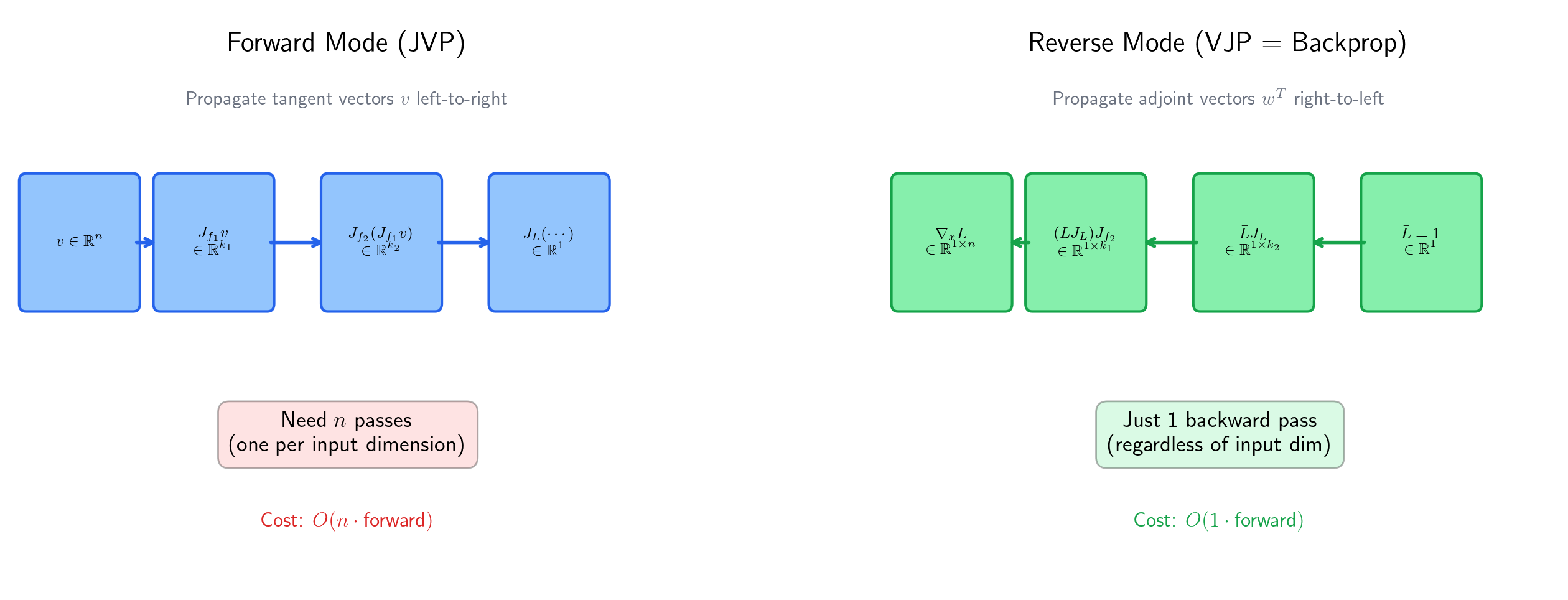
Connections to Statistics
The Jacobian determinant is the volume-scaling factor that makes the change-of-variables formula work for densities. Every transformation of a continuous random variable, every reparameterization of an MCMC sampler, and every score equation in a GLM passes through a Jacobian.
Density transformations
The pushforward formula is a direct application of the multivariate change-of-variables theorem. This is how every transformation of a continuous random variable is analyzed. See formalStatistics Random Variables and formalStatistics Multivariate Distributions.
MCMC reparameterization
Non-centered parameterization with decouples the posterior geometry of hierarchical models. The reparameterization introduces a trivial Jacobian (), making the sampler more efficient. Volume-preservation of leapfrog integration in HMC is a Jacobian-determinant-equals-1 statement. See formalStatistics Bayesian Computation & MCMC.
GLM score and IRLS
The GLM score involves (Jacobian of the mean w.r.t. the linear predictor), and the IRLS weight matrix contains terms. Under the canonical link these simplify, but the Jacobian structure is what makes IRLS general. See formalStatistics Generalized Linear Models.
Connections to ML — Backpropagation & Normalizing Flows
Backpropagation is the multivariate chain rule
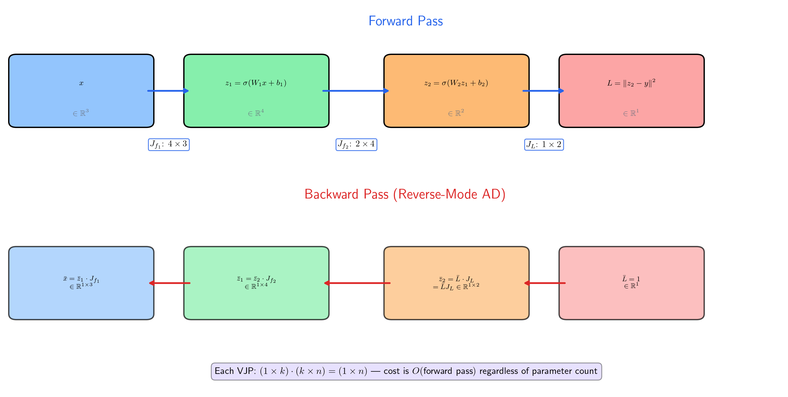
A -layer neural network computes , where each . The loss is . By the chain rule (Theorem 2, applied recursively):
where each is evaluated at the activation from the forward pass. For a scalar loss (), is a row vector — the gradient of with respect to the network output. The gradient with respect to any intermediate layer is obtained by multiplying Jacobians from the loss backward through the chain.
This is not an analogy. Backpropagation is literally the multivariate chain rule, evaluated right-to-left.
Forward mode vs. reverse mode
The product can be evaluated in two orders:
- Right-to-left (forward mode): compute , then , then , and so on. Each step is a JVP. For a scalar loss and parameters, this requires forward passes — one per parameter.
- Left-to-right (reverse mode, backprop): compute , then , then , and so on. Each step is a VJP. For a scalar loss, this requires one backward pass, regardless of .
The asymmetry is dramatic: reverse mode is backward passes for a scalar loss, while forward mode is . This is why we can train networks with billions of parameters.
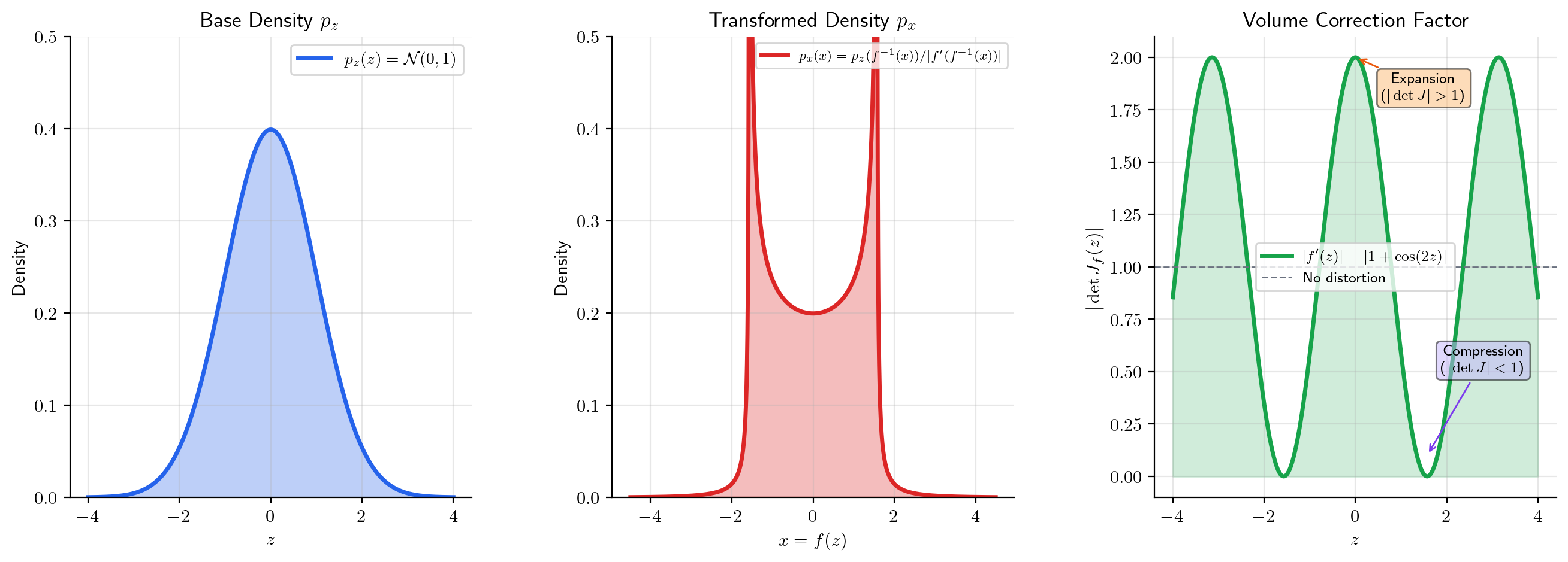
Jacobians in normalizing flows
Normalizing flows transform a simple base density (e.g., a Gaussian) through an invertible function to produce a complex density . By the change-of-variables formula:
or equivalently, . The Jacobian determinant is the “volume correction” that accounts for how stretches or compresses probability mass. Architectures like RealNVP and GLOW use coupling layers with triangular Jacobians, so that is the product of diagonal entries — cheap to compute.
Jacobian regularization
Adding (the squared Frobenius norm of the Jacobian) as a regularization term encourages smoothness: a small Jacobian norm means small sensitivity to input perturbations. From the linear approximation (Proposition 1):
so bounding the Jacobian norm bounds the Lipschitz constant. This appears in adversarial robustness (small perturbations to produce small changes in ), generative models, and physics-informed neural networks.
Forward links to formalML:
- Gradient Descent — backpropagation as the chain rule through computation graphs
- Smooth Manifolds — the Jacobian as the pushforward between tangent spaces
- Information Geometry — the Fisher information matrix transformation under reparametrization via the Jacobian
Connections & Further Reading
Prerequisites — topics you need first
Partial Derivatives & the Gradient
The gradient ∇f(a) of a scalar-valued function is a special case of the Jacobian: when m = 1, the Jacobian is a 1 × n row matrix, and its transpose is the gradient vector. Everything from Topic 9 — partial derivatives, the total derivative, the C¹ criterion — extends directly to the vector-valued setting.
The Derivative & Chain Rule
The single-variable chain rule (f∘g)'(a) = f'(g(a)) · g'(a) from Topic 5 is the 1 × 1 case of the multivariate chain rule J_{f∘g}(a) = J_f(g(a)) · J_g(a). The conceptual insight is the same — the derivative of a composition is the product of the derivatives — but the product becomes matrix multiplication.
Epsilon-Delta & Continuity
The total derivative definition uses a multivariable limit (‖h‖ → 0 in ℝⁿ), and the chain rule proof requires careful ε-δ management of the error terms from two composed total derivatives.
Completeness & Compactness
Compactness arguments ensure that continuous functions on compact domains achieve extrema, used implicitly when discussing global properties of differentiable maps.
Where this leads — next in formalCalculus
On to formalStatistics — where this calculus powers inference
Random Variables
Transformations Y = g(X) of continuous random variables use the change-of-variables formula f_Y(y) = f_X(g⁻¹(y)) · |det J_{g⁻¹}(y)|. The Jacobian determinant is the local volume-scaling factor that makes the density transformation law work.
Multivariate Distributions
The multivariate change-of-variables formula for densities requires the Jacobian of the transformation. Polar-to-Cartesian, spherical coordinates, and linear transformations of the multivariate Normal all invoke Jacobian determinants.
Bayesian Computation And MCMC
Non-centered parameterization (θ = μ + σ·z with z ~ N(0,1)) decouples the posterior geometry of hierarchical models. The reparameterization introduces a trivial Jacobian (σ), making the sampler more efficient. Volume-preservation of leapfrog integration in HMC is a Jacobian-determinant-equals-1 statement.
Generalized Linear Models
The GLM score involves ∂μ/∂η (Jacobian of the mean w.r.t. the linear predictor), and the IRLS weight matrix W contains (∂μ/∂η)² terms. Under the canonical link these simplify, but the Jacobian structure is what makes IRLS general.
On to formalML — where this calculus powers ML
Gradient Descent
Backpropagation computes ∇L by applying the multivariate chain rule through each layer of the network. The Jacobian of each layer is multiplied in sequence: J_{L∘fₖ∘⋯∘f₁} = J_L · J_fₖ ⋯ J_f₁. Reverse-mode AD evaluates this product right-to-left via vector-Jacobian products, computing the full gradient in O(1) backward passes regardless of parameter count.
Smooth Manifolds
The Jacobian of a smooth map f: M → N between manifolds is the pushforward map df_p: T_pM → T_{f(p)}N between tangent spaces. The chain rule d(g∘f)_p = dg_{f(p)} ∘ df_p is the functoriality of the tangent functor.
Information Geometry
The Fisher information matrix transforms under reparametrization φ via I(φ(η)) = J_φᵀ I(η) J_φ — a Jacobian sandwich expressing how the natural Riemannian metric on a statistical manifold changes under coordinate transforms.
Bayesian Neural Networks
The Hessian of the negative log-posterior — central to Laplace approximation in §3.1 — is a Jacobian of the gradient field, and KFAC / diagonal-Fisher reductions in §3.4 are structured Jacobian approximations that scale Bayesian deep learning to modern parameter counts.
Meta Learning
MAML's outer-loop meta-gradient is a Jacobian-of-Jacobian: the chain rule applied through the unrolled inner-loop SGD trajectory (§§2.4–2.6). The Pearlmutter (1994) Hessian-vector-product identity §2.7 is a direct calculation in the vector-valued chain-rule framework developed here.
Normalizing Flows
Flow architectures are engineered around the Jacobian determinant: coupling layers (§4) and autoregressive flows (§5) impose triangular Jacobian structure so that $\log|\det \partial T/\partial z|$ is computable in $O(d)$ time instead of $O(d^3)$. Every flow's log-density formula is downstream of the Jacobian-determinant change-of-variables identity.
Probabilistic Programming
§3 computes Jacobians for the log, logit, and stick-breaking transforms throughout. The Jacobian-as-linearization view and the determinant-as-local-volume-scaling interpretation — both essential for understanding why the Jacobian factor appears in (3.1) — sit on the framework developed in this topic.
Reversible Jump MCMC
The Jacobian determinant of the auxiliary-variable bijection $T_m$ is the unit-conversion factor that makes the trans-dimensional acceptance ratio dimensionally consistent across fibers of different dimensions. §§5–8 use this throughout; the master acceptance ratio in §7 absorbs $|\det J_T|$ as the new ingredient versus fixed-dim MH.
Riemann Manifold Hmc
RMHMC's volume-preservation theorem rests on a Jacobian-determinant calculation for the generalized leapfrog map, and the Metropolis correction is a change-of-variables on the augmented $(\theta, p)$ state space that uses the multivariate Jacobian directly.
Sequential Monte Carlo
Resampling and kernel-mutation moves preserve the weighted empirical measure under coordinate change; the Jacobian of the transform appears in the reweighting calculation whenever a propagation kernel reparametrizes the state space, and the bisection-based adaptive schedule's monotonicity argument uses Jacobian-of-CDF reasoning.
Stochastic Gradient MCMC
The Riemann-manifold metric tensor $G(\theta)$ in §10 is a smooth assignment of positive-definite matrices to points in parameter space; computing its inverse and divergence requires the Jacobian-style multivariable-calculus machinery developed in this topic.
Variational Inference
The change-of-variables formula in §5.3's normalizing-flow constructions is a Jacobian computation; coupling layers are engineered so the Jacobian determinant is triangular, making $\log|\det J|$ cheap to evaluate and the ELBO tractable for richer variational families.
References
- book Munkres (1991). Analysis on Manifolds Chapters 2–3 develop the total derivative and the chain rule in ℝⁿ with full rigor — the primary reference for this topic's proof of the multivariate chain rule
- book Spivak (1965). Calculus on Manifolds Chapter 2 treats the derivative as a linear map and proves the chain rule in the most general finite-dimensional setting — elegant and minimal
- book Rudin (1976). Principles of Mathematical Analysis Chapter 9 on multivariable differentiation — Theorem 9.15 is the chain rule with a clean proof via the contraction mapping characterization of the derivative
- book Axler (2024). Linear Algebra Done Right Determinants, linear maps, and matrix multiplication — the linear algebra foundation for understanding the Jacobian as a matrix representation of a linear map
- book Goodfellow, Bengio & Courville (2016). Deep Learning Section 6.5 on backpropagation — the chain rule applied to computation graphs, forward-mode vs. reverse-mode AD
- paper Rezende & Mohamed (2015). “Variational Inference with Normalizing Flows” Normalizing flows use the change-of-variables formula with the Jacobian determinant to compute densities of transformed distributions — the probabilistic application of the Jacobian determinant
- paper Baydin, Pearlmutter, Radul & Siskind (2018). “Automatic Differentiation in Machine Learning: a Survey” Comprehensive survey of forward-mode and reverse-mode AD — the computational realization of the chain rule in modern ML frameworks