Change of Variables & the Jacobian Determinant
Transforming integrals under coordinate substitution — the Jacobian determinant as the volume scaling factor, polar, cylindrical, and spherical coordinates, the Gaussian integral, and density transformations in normalizing flows
Abstract. The change of variables formula transforms a multiple integral from one coordinate system to another: if φ: D* → D is a C¹ diffeomorphism, then ∫∫_D f(x,y) dA = ∫∫_{D*} f(φ(u,v)) |det J_φ(u,v)| du dv. The Jacobian determinant |det J_φ| measures how φ distorts area elements — it is the volume scaling factor that was introduced abstractly in the Jacobian topic and now does real computational work. Polar coordinates are the canonical example: the map (r,θ) → (r cos θ, r sin θ) has Jacobian determinant r, producing the area element r dr dθ. This immediately resolves the painful disk integral from Topic 13 and enables the classic proof that the Gaussian integral equals √π — a result that propagates throughout probability and statistical mechanics. Cylindrical and spherical coordinates extend the framework to three dimensions. The general theorem, proved via the Inverse Function Theorem and a partition of unity argument, guarantees that integration is coordinate-independent for any C¹ diffeomorphism. In machine learning, the change of variables formula is the mathematical engine of normalizing flows: the density of a transformed variable X = f(Z) satisfies p_X(x) = p_Z(f⁻¹(x)) · |det J_{f⁻¹}(x)|, and the entire architecture of flow-based generative models is designed to make this Jacobian determinant tractable. The reparameterization trick in variational autoencoders is the same formula applied to move gradient computation outside the expectation.
1. Overview & Motivation
You’ve built a generative model — a neural network that maps simple noise to complex data . To train it, you need the density . The change of variables formula gives it:
The entire architecture of normalizing flows is designed to make the right side of this equation tractable. And the formula itself — “adjust the density by the Jacobian determinant” — is exactly the integration change of variables from multivariable calculus, applied to probability.
This topic brings together the Jacobian determinant (Topic 10), the Inverse Function Theorem (Topic 12), and multiple integrals (Topic 13) into a single powerful formula. The reader already has all the ingredients; this topic assembles them.
2. Substitution in One Variable — The Template
We know -substitution from Topic 7, but we reframe it through the lens of coordinate transformation to set up the multivariable version.
🔷 Theorem 1 (Substitution Rule (1D))
Let be a bijection with on . Then for any continuous :
The factor adjusts for how stretches or compresses the interval. When is increasing, ; when decreasing, , which also reverses the limits to compensate.
💡 Remark 1 (Why the Absolute Value?)
In 1D, you can track orientation via limit ordering. In , there are no “limits” to reverse — the absolute value of the Jacobian determinant is the only way to ensure positivity of the volume element. The absolute value is the conceptual bridge from 1D to D.
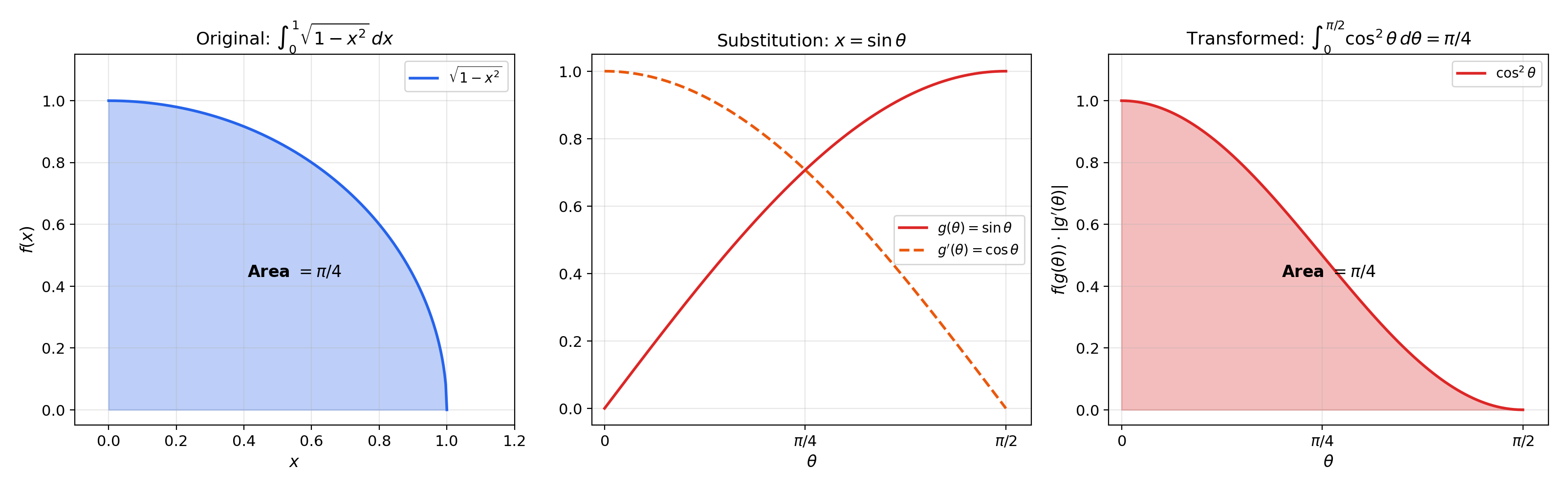
📝 Example 1 (Quarter-Circle Area via Substitution)
Compute via . We have , , limits :
This is one quarter of the unit disk area — a preview of polar coordinates.
📝 Example 2 (Gaussian Integral via Gamma Function)
Compute via . We get , :
This connects to the Gamma function (Topic 8) and previews the Gaussian integral computation later in this topic.
3. The Change of Variables Formula in 2D
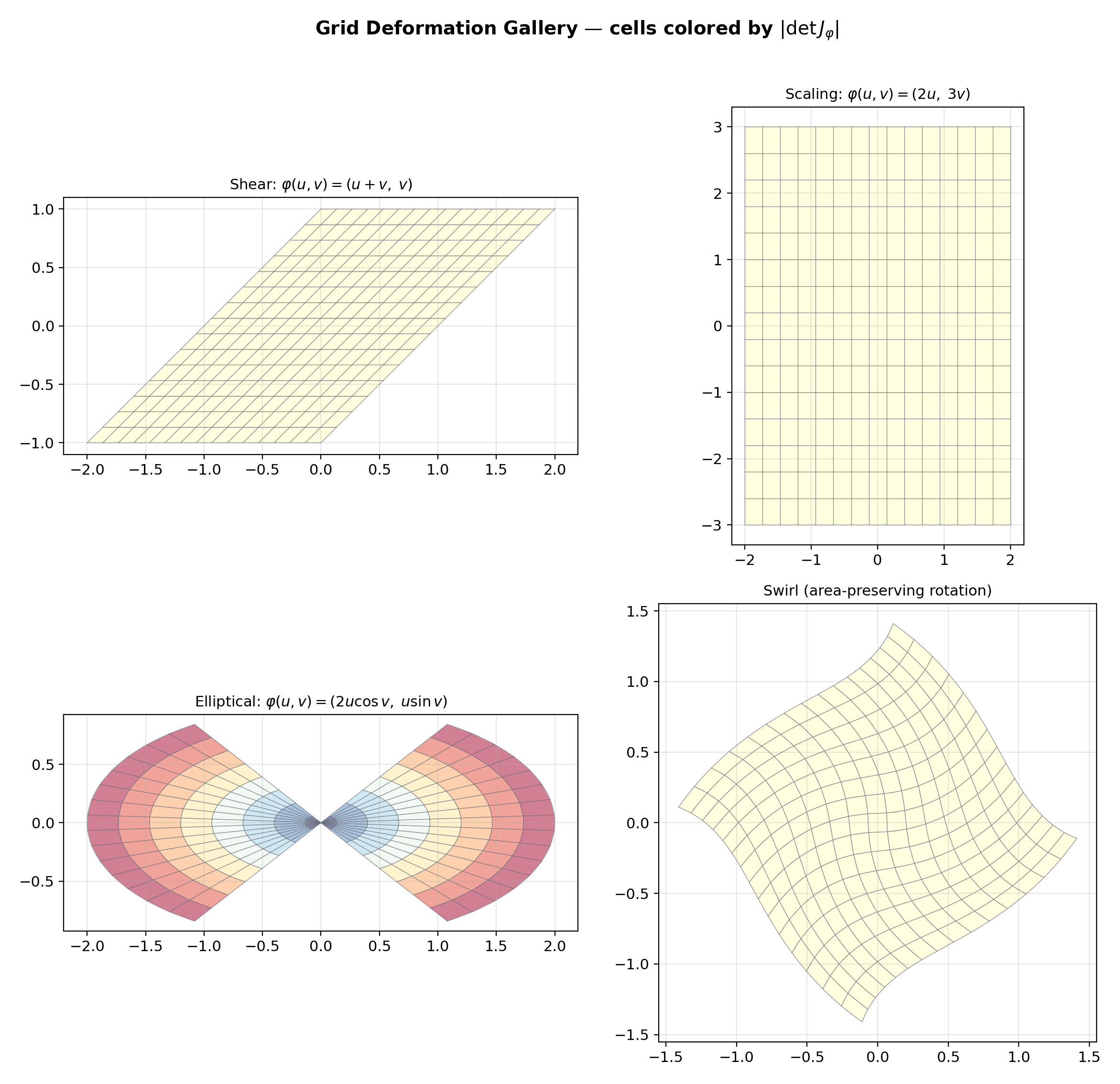
This is where the Jacobian determinant enters integration. Draw a grid in the -plane. The map sends each small rectangle to a small parallelogram in the -plane. The area of that parallelogram is approximately — this is exactly the Volume Distortion Theorem from Topic 10. The change of variables formula says: sum up over the deformed parallelograms, weighting each by its area.
📐 Definition 1 (Coordinate Transformation)
A coordinate transformation (or change of variables) on an open set is a function that is a diffeomorphism: bijective, , and with inverse .
💡 Remark 2 (Diffeomorphism vs. Local Diffeomorphism)
The IFT (Topic 12) guarantees a local diffeomorphism wherever . For the change of variables formula, we need a global diffeomorphism on (or at least injectivity, with only on a set of measure zero). Polar coordinates fail to be a global diffeomorphism on because of the -periodicity in , but they are a diffeomorphism on any domain that doesn’t wrap all the way around.
🔷 Theorem 2 (Change of Variables (2D))
Let be a diffeomorphism between open subsets of , and let be continuous. Then:
The Jacobian determinant converts the area element in the -coordinate system to the area element in the -coordinate system.
📝 Example 3 (Linear Change of Variables)
For with and : (constant). The formula reduces to . Linear maps scale all areas by the same factor.
📝 Example 4 (Affine Shear)
For : . The integral is unchanged: . Area-preserving transformations have a unit Jacobian determinant.
💡 Remark 3 (The Formula in Reverse)
Often we start with an integral in and want to transform to . If is the transformation , then we substitute , , , and change the region from to . The conceptual direction is: “I want simpler limits, so I find a that maps a simple to the complicated .”
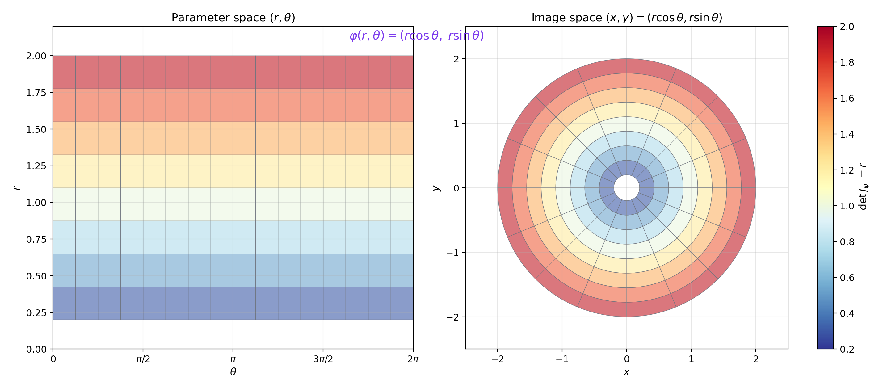
Polar coordinates: (r,θ) → (r cos θ, r sin θ). The Jacobian determinant is r — cells near the origin are compressed.
|det J| range: [0.179, 1.921]
4. Polar Coordinates
The reader has been waiting for this since Example 7 of Topic 13 (the disk integral that was “painful in Cartesian”). Polar coordinates are the prototypical 2D change of variables.
📐 Definition 2 (Polar Coordinates)
The polar coordinate transformation is , mapping from to (the plane minus the positive -axis). The Jacobian is:
The area element is .
💡 Remark 4 (Why r > 0?)
At , , and collapses all values to the origin — it is not injective. The origin is a single point (measure zero), so excluding it does not affect the integral. This is typical: changes of variables are allowed to fail on sets of measure zero.
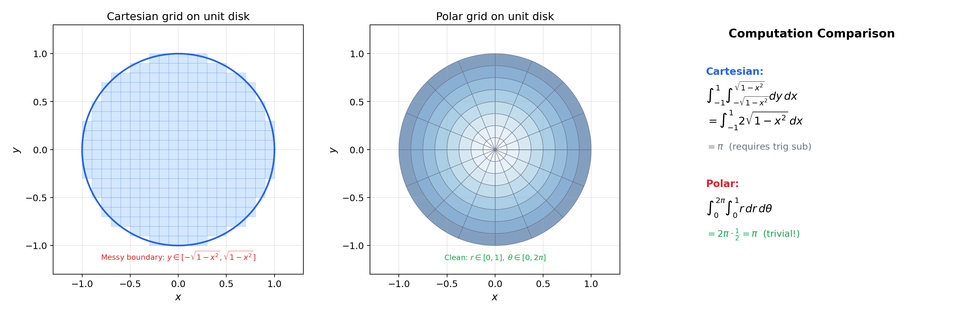
📝 Example 5 (Area of the Unit Disk (Resolved))
Compare with the Cartesian computation from Topic 13, Example 7: . Same answer, but polar reduces the integral to a product of two elementary 1D integrals.
📝 Example 6 (Integral over an Annulus)
over the annulus : in polar, :
The circular symmetry of both the region and the integrand makes polar coordinates the natural choice.
📝 Example 7 (Volume Under the Paraboloid (Resolved))
From Topic 13, §7: the volume between and over the disk . In polar:
Polar Riemann sum: 3.141593 | Exact: 3.141593 | Error: 4.44e-16
5. The Gaussian Integral
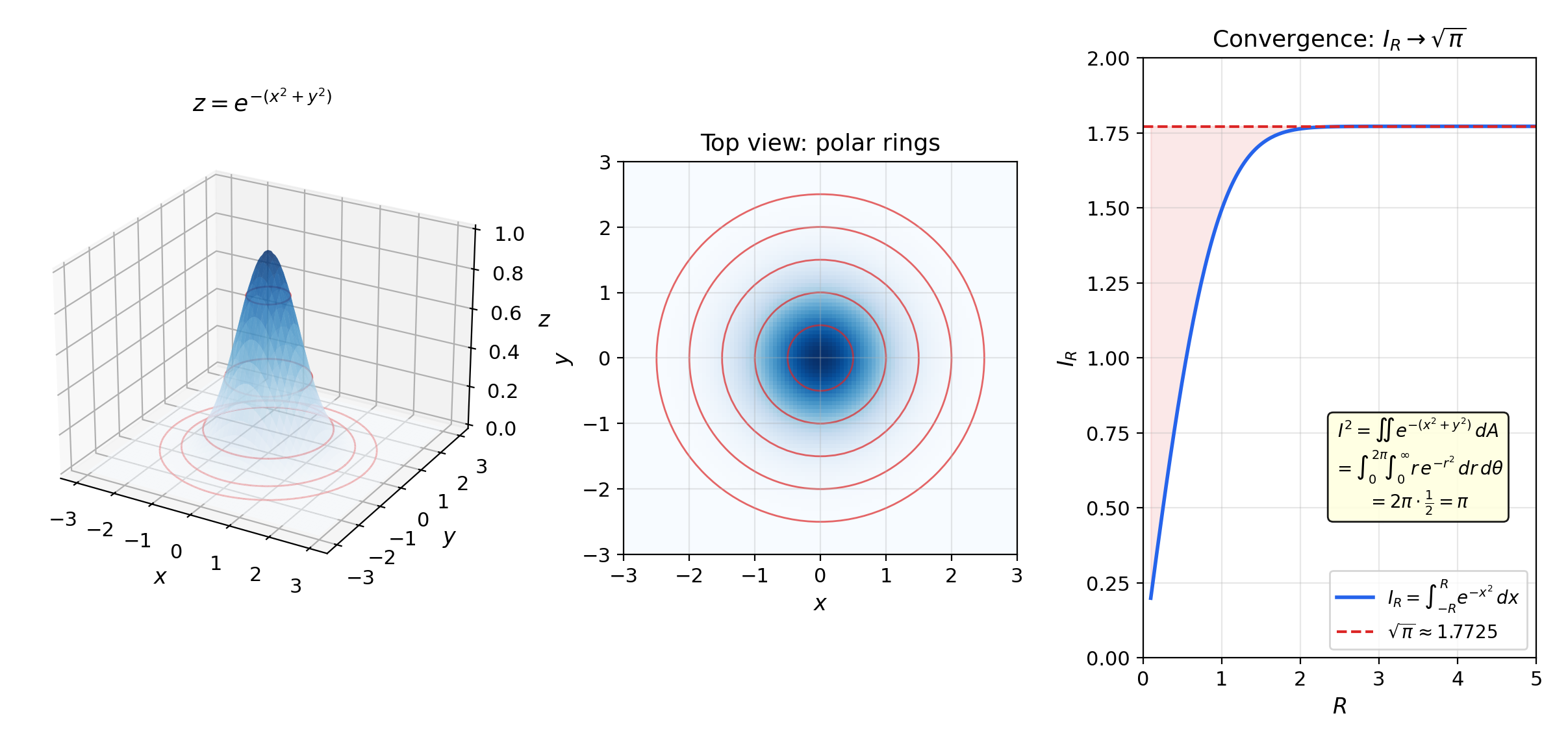
The computation of is one of the most important results in all of mathematics, appearing in probability (the normalizing constant of the normal distribution), statistical mechanics (the partition function), and quantum mechanics (path integrals). The proof is a triumph of the change-of-variables formula.
🔷 Proposition 1 (The Gaussian Integral)
Proof.
Step 1: Square the integral. Let . Then:
The first equality uses Fubini (Topic 13, Theorem 1) to convert the product of two 1D integrals into a double integral. This requires justifying that is integrable over — it suffices to note that as , so the improper integral converges.
Step 2: Switch to polar coordinates. Using and :
The inner integral is elementary: .
Step 3: Evaluate. . Since , we conclude .
💡 Remark 5 (Why Is This Hard in Cartesian?)
The function has no elementary antiderivative (this is a theorem, not a failure of technique). The 1D integral is genuinely intractable without the 2D “trick.” The change-of-variables formula transforms a hard 1D problem into an easy 2D one by exploiting radial symmetry.
📝 Example 8 (The Gaussian Normalizing Constant)
The PDF of is . Verify normalization using the substitution and :
This is why the appears in the Gaussian density — it is the Gaussian integral.
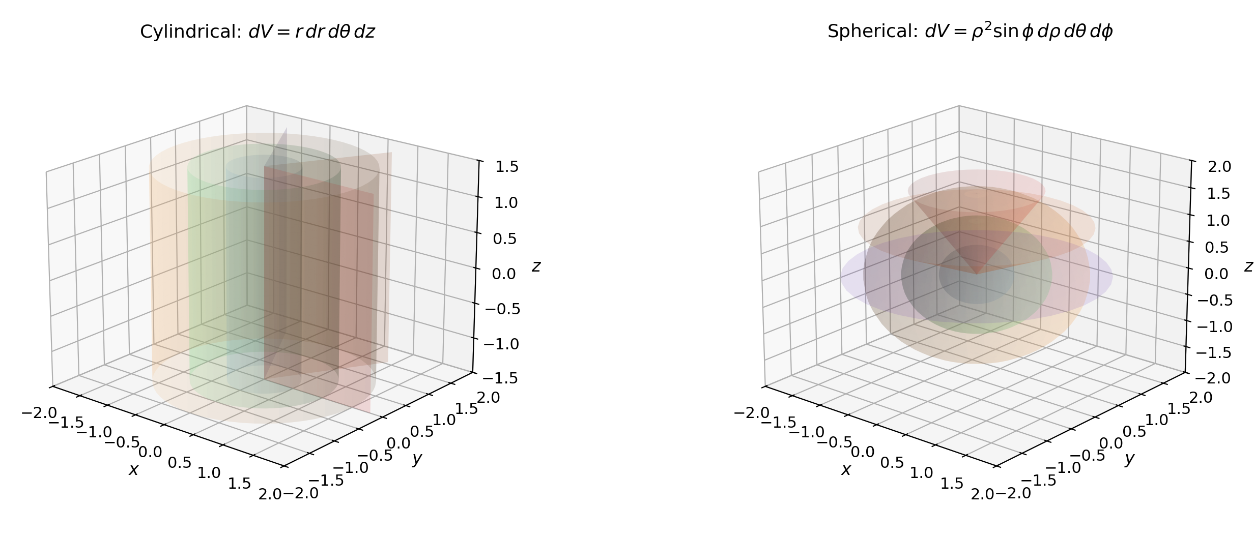
6. Cylindrical and Spherical Coordinates
The change of variables formula works in any dimension. Here we cover the two standard 3D coordinate systems.
📐 Definition 3 (Cylindrical Coordinates)
The cylindrical coordinate transformation is , with , , . The Jacobian is:
The volume element is .
📐 Definition 4 (Spherical Coordinates)
The spherical coordinate transformation is , with , , . The Jacobian matrix is:
Computing by cofactor expansion along the third row:
Since for : . The volume element is .
📝 Example 9 (Volume of the Unit Ball)
Three decoupled 1D integrals — the spherical symmetry of the ball makes the computation trivial.
📝 Example 10 (Moment of Inertia of a Solid Sphere)
For a uniform solid sphere of mass and radius with density , the moment of inertia about the -axis is . In spherical coordinates, :
Evaluating each factor: , , . So .
💡 Remark 6 (Which Coordinate System to Use?)
- Polar: circular symmetry in 2D ( appears, region is a disk or annulus).
- Cylindrical: cylindrical symmetry in 3D (the region or integrand is symmetric about the -axis).
- Spherical: spherical symmetry ( appears, region is a ball or spherical shell).
- If none of these symmetries are present, a custom coordinate transformation may still simplify the integral.
(ρ, θ, φ) = (1.00, 1.05, 0.79) | |det J| = 0.7071
■ const-ρ ■ const-θ ■ const-φ ■ volume element
7. The General Change of Variables Theorem
Polar, cylindrical, and spherical are special cases. The general theorem handles any diffeomorphism.
📐 Definition 5 (C¹ Diffeomorphism)
A function between open subsets of is a diffeomorphism if: (i) is bijective, (ii) is (continuously differentiable), and (iii) is . By the Inverse Function Theorem (Topic 12, Theorem 1), conditions (ii) and (iii) are equivalent to: is and for all .
🔷 Theorem 3 (Change of Variables (General))
Let be a diffeomorphism between open subsets of . Let be continuous and integrable over . Then:
This reduces to the 1D substitution rule (Theorem 1) when , and to the 2D formula (Theorem 2) when .
Proof.
We follow Spivak’s approach (Calculus on Manifolds, Theorem 3-13).
Step 1: The linear case. If is an affine map with invertible, then , , and the formula follows from the definition of the Riemann integral: the Riemann sum over with partition corresponds to the Riemann sum over with partition , with each cell volume scaled by .
Step 2: Local validity. For a general diffeomorphism and any , the linear approximation is accurate on a small ball . Because is continuous and , on a sufficiently small ball:
for any prescribed . The integral formula holds locally up to an error controlled by .
Step 3: Partition of unity. Cover with a finite collection of balls (using compactness of if is bounded; the general case uses exhaustion by compact subsets — see Topic 3 for compactness). Choose a subordinate partition of unity : smooth functions with and on . Then:
Each step uses: (i) the partition of unity decomposes into locally supported pieces, (ii) the linear case applies locally on each (up to the error in Step 2), (iii) summing recovers the full integral. The rigorous details involve showing the error terms from Step 2 sum to zero — this uses the uniform continuity of on compact subsets.
💡 Remark 7 (Relaxing the Hypotheses)
The theorem extends to that fails to be injective or has on a set of measure zero (e.g., the origin for polar coordinates, or the -axis for cylindrical coordinates). The Lebesgue version of the change-of-variables theorem handles this rigorously — see Sigma-Algebras & Measures and The Lebesgue Integral (coming soon).

8. A Gallery of Coordinate Transformations
This section builds computational fluency through a series of worked examples with different transformations.
📝 Example 11 (Elliptical Coordinates — Area of an Ellipse)
Let with . The Jacobian determinant is . The area of the ellipse :
This generalizes the disk area to .
📝 Example 12 (Parabolic Coordinates)
has . Useful for problems with parabolic symmetry (e.g., electrostatics near a parabolic reflector).
🔷 Proposition 2 (Composition of Transformations)
If and are diffeomorphisms, then is a diffeomorphism with:
This follows from the chain rule for Jacobians (Topic 10, Theorem 2) and the multiplicativity of determinants. Geometrically: volume distortions compose multiplicatively, as established in Topic 10, Proposition 2.
📝 Example 13 (Composed Transformation — Rotated Ellipse)
To integrate over the region (a rotated ellipse), first rotate by to diagonalize the quadratic form, then scale to a unit disk. The composed Jacobian determinant is the product of the individual determinants.
9. The Density Transformation Formula
This section reframes the change of variables formula for probability densities and connects to normalizing flows — the most direct ML application of this calculus.
📐 Definition 6 (Density Transformation)
Let be a random vector with density and let where is a diffeomorphism. The density of is:
This follows directly from the change of variables theorem applied to for all measurable .
📝 Example 14 (Log-Normal from Normal)
If and , then , , . So:
This is the log-normal density.
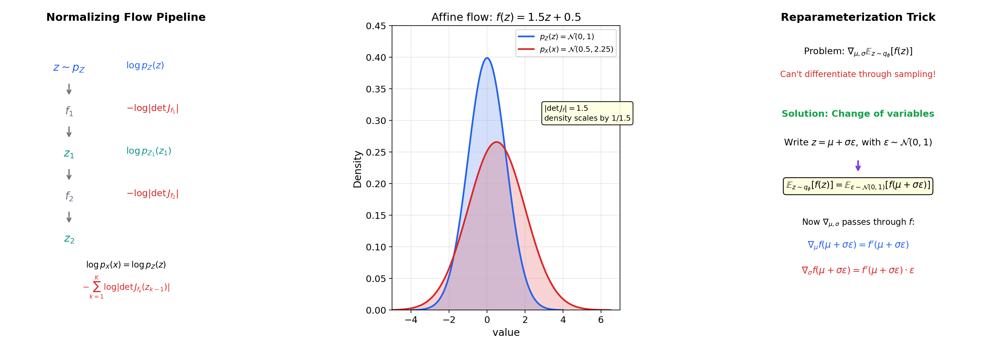
💡 Remark 8 (Normalizing Flows)
A normalizing flow is a composition of diffeomorphisms: . By the composition rule (Proposition 2):
where and . The entire architecture of flow-based generative models (RealNVP, Glow, Neural Spline Flows) is designed to make each cheap to compute — typically instead of — by using triangular Jacobians (coupling layers, autoregressive transforms). This is the change-of-variables formula doing heavy lifting in generative modeling.
📝 Example 15 (Affine Coupling Layer (RealNVP))
The RealNVP coupling layer splits and defines , . The Jacobian is lower-triangular with diagonal entries (for ) and (for ). So — a sum, not a determinant. This is and trivially differentiable. The IFT (Topic 12) guarantees invertibility since everywhere.
💡 Remark 9 (The Reparameterization Trick)
In variational autoencoders, we need where . The expectation depends on through the distribution, so we can’t just differentiate under the integral sign. The trick: write with . This is a change of variables from to . Now , and the gradient moves inside: is just a standard derivative of a deterministic function of evaluated at a random . The change-of-variables formula separates the randomness () from the parameters ().
∫p_X(x)dx ≈ 1.0000
Connections & Further Reading
Prerequisites — topics you need first
Inverse & Implicit Function Theorems
The change of variables formula requires φ to be a C¹ diffeomorphism — locally invertible with C¹ inverse. The IFT guarantees this when det J_φ ≠ 0.
Multiple Integrals & Fubini's Theorem
Every integral in this topic is a multiple integral evaluated via Fubini. The disk integral (Example 7 from Topic 13) is resolved here in polar coordinates.
The Jacobian & Multivariate Chain Rule
The Jacobian determinant |det J_φ| as a volume scaling factor was introduced in Topic 10. This topic gives it its computational starring role.
The Riemann Integral & FTC
The 1D substitution rule is the single-variable ancestor. This topic generalizes it from |g'(x)| to |det J_φ|.
Improper Integrals & Special Functions
The Gaussian integral ∫e^{-x²}dx = √π, previewed in Topic 8, is proved here via polar coordinates.
Completeness & Compactness
Compactness of the integration domain ensures the partition of unity is finite in the general proof.
Where this leads — next in formalCalculus
Surface Integrals & the Divergence Theorem
Surface parameterization requires the Jacobian of the parameterization map; the surface area element involves the cross product of tangent vectors, which is the 2D analog of the Jacobian determinant.
The Lebesgue Integral
The Lebesgue change of variables theorem generalizes the Riemann version here, relaxing the diffeomorphism requirement to almost-everywhere injectivity.
Sigma-Algebras & Measures
Pushforward measures and the change-of-variables formula for Lebesgue integrals depend on the Jacobian determinant — the measure-theoretic framework formalizes what this topic does concretely.
On to formalStatistics — where this calculus powers inference
Random Variables
The pushforward density formula f_Y(y) = f_X(g⁻¹(y)) · |det J_{g⁻¹}(y)| is a direct application of the multivariate change-of-variables theorem. This is how every transformation of a continuous random variable is analyzed.
Multivariate Distributions
Polar-to-Cartesian, spherical coordinates, and linear transformations of the multivariate Normal all invoke the change-of-variables theorem. Copula constructions invert the marginal CDFs — another change-of-variables operation.
Bayesian Foundations And Prior Selection
The Jeffreys prior π(θ) ∝ √det I(θ) is constructed to be invariant under reparameterization φ = g(θ) — a property that follows from the Jacobian cancellation in the change-of-variables formula. Invariance is its defining feature.
Continuous Distributions
Lognormal from Normal, Chi-squared from Normal, t from Normal+Chi-squared, F from two Chi-squared — every derived distribution is obtained via change-of-variables on a known density.
On to formalML — where this calculus powers ML
Gradient Descent
The reparameterization trick in variational inference — writing z = μ + σε with ε ~ N(0,1) — is a change of variables that moves parameters outside the expectation, enabling gradient computation through sampling.
Measure Theoretic Probability
The density transformation formula p_X(x) = p_Z(φ⁻¹(x)) · |det J_{φ⁻¹}(x)| is the probabilistic form of the change of variables theorem.
Smooth Manifolds
Integration on manifolds requires coordinate charts, and the change of variables formula ensures that integrals are well-defined independent of chart choice.
Information Geometry
The Fisher information matrix transforms under reparameterization via Ĩ(θ̃) = JᵀI(θ)J, where J is the Jacobian of the parameter change.
Normalizing Flows
Every flow's log-density formula is downstream of the substitution rule $p_X(x) = p_Z(T^{-1}(x)) \cdot |\det \partial T^{-1}/\partial x|$. §2.2's $d$-dimensional version takes the substitution rule as a load-bearing tool, and the architecture's design pressure for triangular Jacobians is exactly to make this formula computationally tractable.
Probabilistic Programming
§3.1's change-of-variables theorem for densities (Theorem 2) is a direct application of the multivariable change-of-variables formula for integrals. The Jacobian-determinant calculation and the substitution argument used in the proof are exactly the pure-calculus moves taught here.
Reversible Jump MCMC
The change-of-variables formula for measurable bijections is the measure-theoretic substrate of §5's Theorem 1 — without it, the push-forward density $q_m$ divided by $|\det J_T|$ isn't well-defined. The inverse-function-theorem corollary $|\det J_{T^{-1}}| = 1/|\det J_T|$ is the algebraic core of §6's reversibility proof.
Sequential Monte Carlo
SMC samplers use a synthetic annealing path $\pi_t \propto \pi_0^{1-\beta}\pi_T^{\beta}$; reparameterization between unconstrained and constrained parameter spaces invokes the change-of-variables theorem and its Jacobian determinant, particularly when propagation kernels operate in reparameterized coordinates.
Sparse Bayesian Priors
§4's horseshoe-shape theorem ($\kappa_j \sim \text{Beta}(\tfrac12, \tfrac12)$ under unit $\tau$) is proved via change-of-variables from $\lambda_j^2$ to $\kappa_j = 1/(1 + \lambda_j^2)$; the Jacobian $d\kappa/d\lambda^2 = 1/\kappa^2$ is computed using the change-of-variables formula. §6's non-centered parameterization $\beta_j = z_j \cdot \lambda_j \cdot \tau$ is also a deterministic change of variables on the hierarchical model.
References
- book Spivak (1965). Calculus on Manifolds Chapter 3, Theorem 3-13 — the change of variables theorem with full proof via partition of unity
- book Rudin (1976). Principles of Mathematical Analysis Theorem 10.9 — change of variables for Riemann integrals in Rⁿ
- book Munkres (1991). Analysis on Manifolds Chapter 3 — change of variables with extended Jacobian and boundary conditions
- book Hubbard & Hubbard (2015). Vector Calculus, Linear Algebra, and Differential Forms Chapter 4 — geometric treatment of coordinate transformations and the Jacobian
- paper Rezende & Mohamed (2015). “Variational Inference with Normalizing Flows” The normalizing flow framework: density transformation via the change of variables formula with tractable Jacobian determinants
- paper Kingma & Welling (2014). “Auto-Encoding Variational Bayes” The reparameterization trick: change of variables applied to move parameters outside the expectation for gradient estimation