Improper Integrals & Special Functions
Extending integration to unbounded intervals and unbounded integrands — the Gamma, Beta, and Gaussian integrals that are workhorses in probability and machine learning
Abstract. The Riemann integral ∫ₐᵇ f(x) dx requires both the interval [a,b] and the function f to be bounded. Improper integrals remove these restrictions by defining ∫ₐ∞ f(x) dx = lim_{b→∞} ∫ₐᵇ f(x) dx (Type I: unbounded intervals) and handling unbounded integrands via one-sided limits at singularities (Type II). The p-test provides the fundamental benchmark: ∫₁∞ 1/xᵖ dx converges if and only if p > 1, while ∫₀¹ 1/xᵖ dx converges if and only if p < 1. Comparison tests — direct and limit — reduce new convergence questions to these benchmarks. Three special functions built from improper integrals pervade probability and machine learning. The Gamma function Γ(s) = ∫₀∞ tˢ⁻¹ e⁻ᵗ dt extends the factorial to real numbers via the functional equation Γ(s+1) = sΓ(s), with Γ(n+1) = n! for positive integers. The Beta function B(a,b) = ∫₀¹ tᵃ⁻¹(1-t)ᵇ⁻¹ dt is the normalizing constant for the Beta distribution, connected to Gamma by B(a,b) = Γ(a)Γ(b)/Γ(a+b). The Gaussian integral ∫₋∞∞ e⁻ˣ² dx = √π normalizes the Gaussian distribution — its proof via polar coordinates is a celebrated application of multivariable substitution. Stirling’s approximation n! ≈ √(2πn)(n/e)ⁿ, derived from the Gamma function, gives the asymptotic behavior of factorials used throughout information theory and combinatorics. In machine learning, these functions appear as normalizing constants for probability distributions (Gaussian, Gamma, Beta, Chi-squared, Student-t), in Bayesian posterior computation, and in the analysis of tail probabilities and concentration inequalities.
Overview & Motivation
You’re computing the normalizing constant for a Gaussian distribution: . This integral has no closed-form antiderivative — has no elementary antiderivative at all. Yet the integral equals , a fact that makes the entire Gaussian probability framework possible. More immediately: every density must satisfy , but this is an integral over an unbounded interval — the Riemann integral from Topic 7 doesn’t apply directly.
Improper integrals make these computations rigorous by defining integrals over unbounded domains (and of unbounded functions) as limits of the proper integrals we’ve already built. The idea is simple: if you can’t integrate all the way to infinity, integrate to some large number and ask what happens as . If the limit is finite, the improper integral converges and we call that limit the value of the integral. If not, the integral diverges.
We’ll extend the Riemann integral to unbounded intervals (§2) and unbounded integrands (§3), develop convergence tests that determine convergence without computing exact values (§4), then meet the three special functions that pervade probability and ML: the Gamma function (§5), the Beta function (§6), and the Gaussian integral (§7). Stirling’s approximation (§8) gives the asymptotic behavior of that appears throughout information theory and combinatorics.
Type I — Integration over Unbounded Intervals
Start with the picture: on . The curve drops toward zero, and we want the total area under it from to the right forever. We can compute for any finite using the FTC. As , this approaches . The area under an infinitely long curve is finite — this is the central surprise of improper integrals.
📐 Definition 1 (Type I Improper Integral)
If is Riemann integrable on for every , we define
provided the limit exists. If the limit exists and is finite, the improper integral converges; otherwise it diverges.
Similarly, , and for doubly infinite integrals:
for any , provided both pieces converge. The choice of doesn’t matter when both parts converge — this follows from the additivity of the Riemann integral over adjacent intervals.
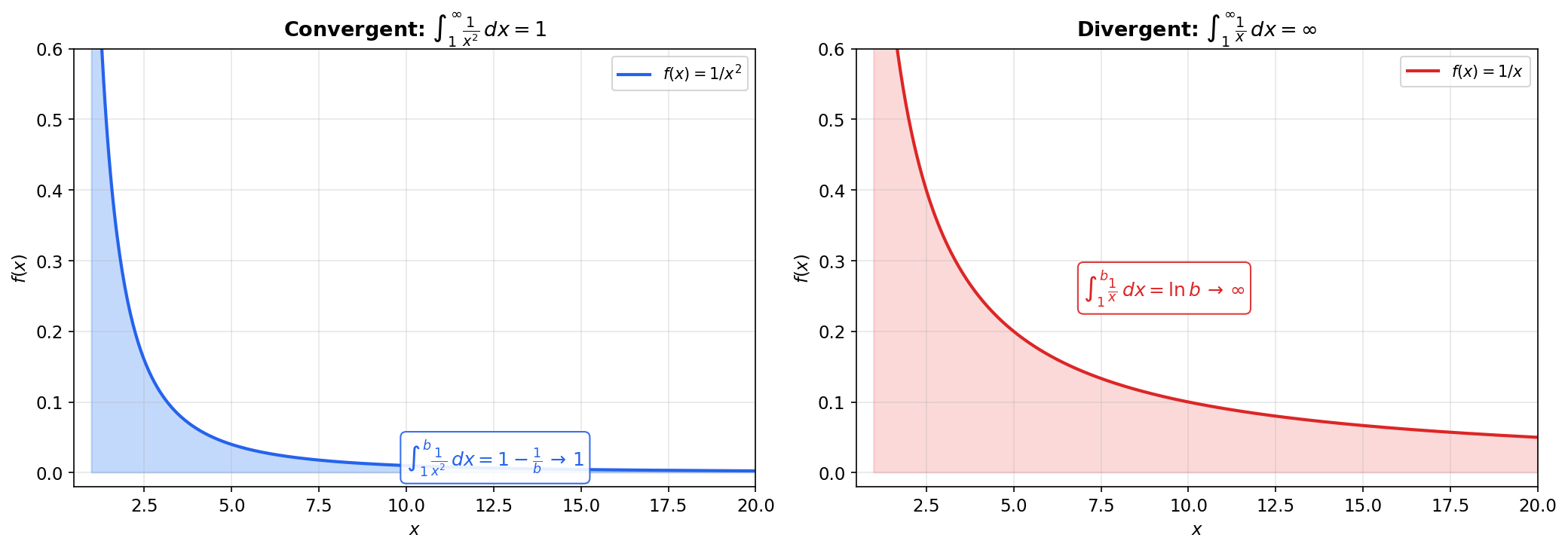
📝 Example 1 (The p-test for Type I)
The integral is the fundamental benchmark for convergence at infinity.
For :
- If : the exponent , so as . The integral converges to .
- If : the exponent , so . The integral diverges.
For : . Diverges.
The integral converges if and only if . This is the -test — every other Type I convergence question reduces to comparing against .
📝 Example 2 (Exponential decay)
Exponential decay is more than fast enough to make the area finite. In fact, decays faster than any power , which is why exponential tails are so well-behaved in probability.
📝 Example 3 (Harmonic divergence)
The harmonic function decays, but too slowly — the area accumulates without bound. This is the borderline case of the -test, and it’s the continuous analog of the divergent harmonic series .
💡 Remark 1 (Doubly improper integrals and the Cauchy principal value)
For , we split at any finite and require both and to converge independently. The Cauchy principal value is a weaker notion — it can exist even when the improper integral diverges. For example, has Cauchy principal value (by symmetry: for all ), but the improper integral diverges because .
p = 2 > 1, so the integral converges to 1/(p−1) = 1
Type II — Integration of Unbounded Functions
Now consider on . The function is unbounded near — it blows up to infinity. Yet the area under the curve from to is , which approaches as . An infinitely tall region can have a finite area — the dual surprise to Type I.
📐 Definition 2 (Type II Improper Integral)
If is Riemann integrable on for every but is unbounded near , we define
provided the limit exists. Similarly, if is unbounded near :
For singularities at an interior point , we split: , and both limits must exist independently.
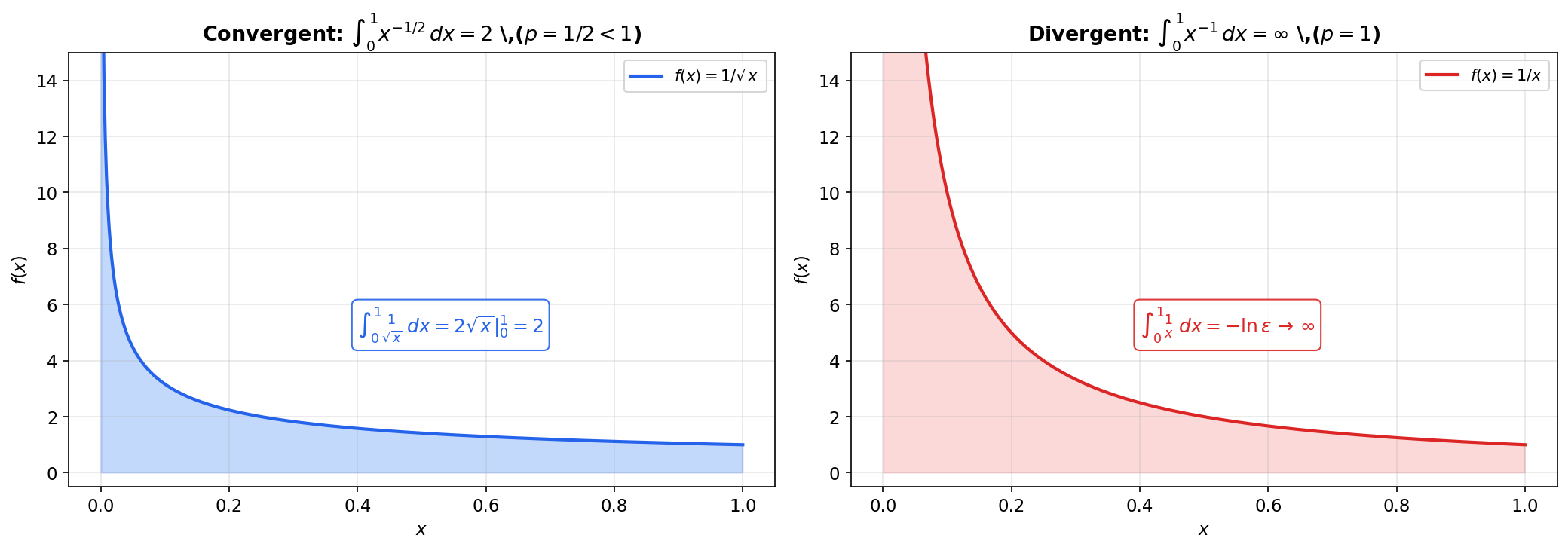
📝 Example 4 (The p-test for Type II)
The integral is the benchmark for convergence near a singularity.
For :
- If : as (since ). The integral converges to .
- If : . The integral diverges.
For : . Diverges.
The integral converges if and only if . Note the complementary relationship with the Type I -test: for convergence at infinity, for convergence at zero. The borderline diverges in both cases.
📝 Example 5 (Square root singularity)
: here , so the integral converges. Explicitly:
The area under on is finite () despite the function blowing up at .
💡 Remark 2 (Interior singularities)
If has a singularity at , we split: , and both parts must converge independently. For example:
Each piece converges (), so the integral converges. The total value is .
💡 Remark 3 (Both types simultaneously)
Some integrals involve both an unbounded interval and an unbounded integrand. For example, has a Type II singularity at (where blows up) and requires a Type I analysis as (where the integrand decays like ). Split at and handle each piece separately: near , compare with (, converges); at infinity, compare with (, converges). The integral converges and equals .
Convergence Tests
The -test is a powerful benchmark, but we need tools to determine convergence for integrals that aren’t exactly . The comparison tests reduce new convergence questions to known ones.
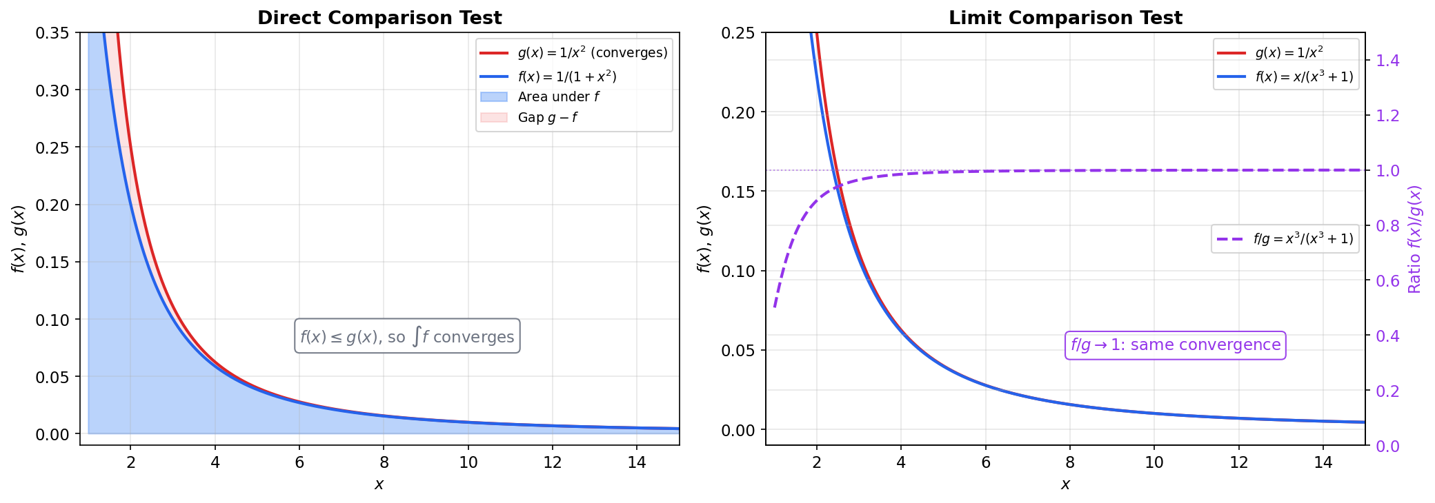
🔷 Theorem 1 (Comparison Test (Direct))
Suppose for all .
(a) If converges, then converges, and .
(b) If diverges, then diverges.
The analogous result holds for Type II integrals.
Proof.
For part (a): let and . By monotonicity of the Riemann integral (Topic 7, Theorem 3), implies for all . Since , the function is increasing in : adding more non-negative area can only increase the integral. Since , the function is increasing and bounded above. By the Monotone Convergence principle (Topic 3), exists and is finite.
Part (b) is the contrapositive of part (a): if converged, then would converge too, contradicting the hypothesis.
📝 Example 6 (Convergence by comparison)
converges. For :
and converges (). By the comparison test, converges.
In fact, we can compute the exact value: .
🔷 Theorem 2 (Limit Comparison Test)
Suppose and for , and .
- If : and either both converge or both diverge.
- If and converges: then converges.
- If and diverges: then diverges.
Proof.
For the case : choose . There exists such that for :
which gives for . Apply the direct comparison test:
- If converges: , so converges by comparison with .
- If diverges: , so diverges.
The cases and follow by similar comparison arguments using one-sided bounds.
📝 Example 7 (Limit comparison in action)
converges. Compare with :
Since and converges, the limit comparison test gives convergence. We didn’t need to compute the integral — knowing its asymptotic behavior was enough.
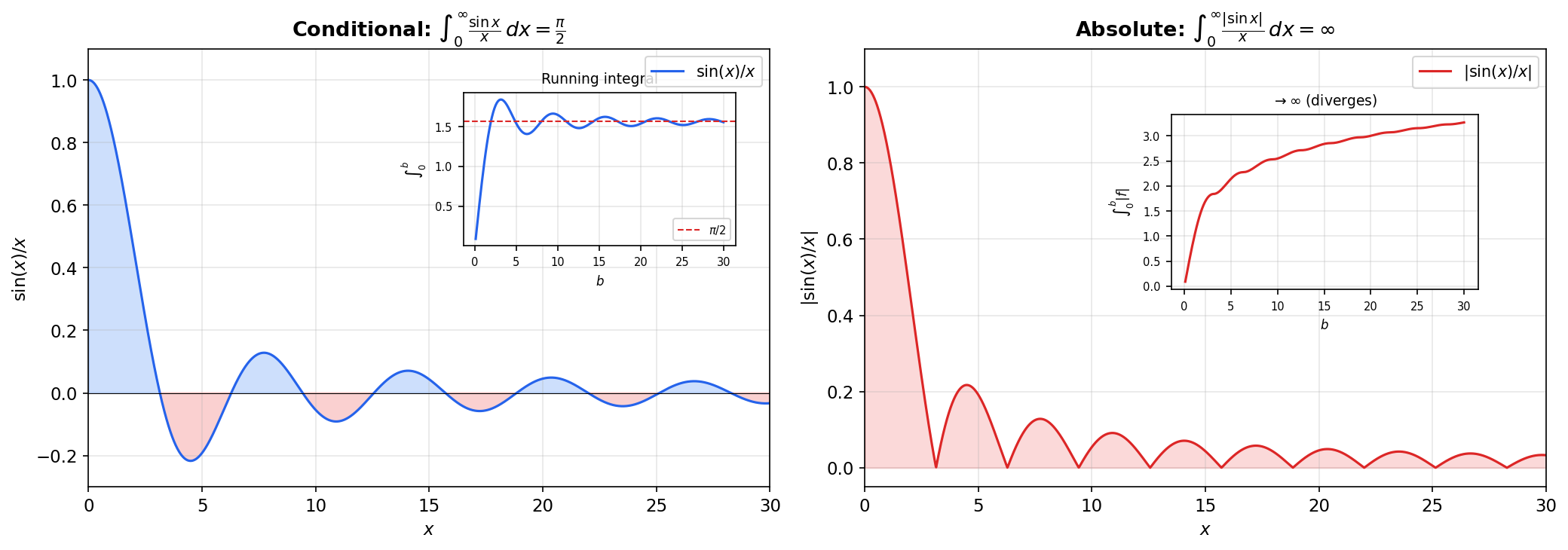
📐 Definition 3 (Absolute and Conditional Convergence)
An improper integral converges absolutely if converges. It converges conditionally if converges but diverges.
🔷 Theorem 3 (Absolute Convergence Implies Convergence)
If converges, then converges, and
Proof.
Write where and . Then , and , . Since converges, both and converge by the comparison test (Theorem 1). Then converges.
The inequality follows: .
📝 Example 8 (The Dirichlet integral converges conditionally)
The Dirichlet integral is a famous result (proved via contour integration or Laplace transforms — we state it without proof here). But diverges: on each interval ,
and diverges (harmonic series). The integral converges conditionally but not absolutely — positive and negative oscillations cancel just enough to produce a finite result, but the total variation is infinite.
💡 Remark 4 (Comparison tests for Type II)
The comparison and limit comparison tests apply to Type II improper integrals with the obvious modifications: compare behavior near the singularity instead of at infinity. For with a singularity at , compare to as ; the -test ( for convergence) provides the benchmark.
The Gamma Function
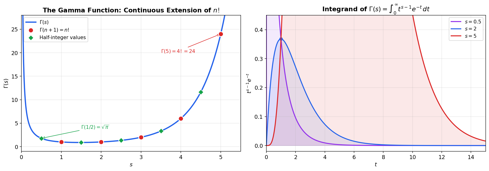
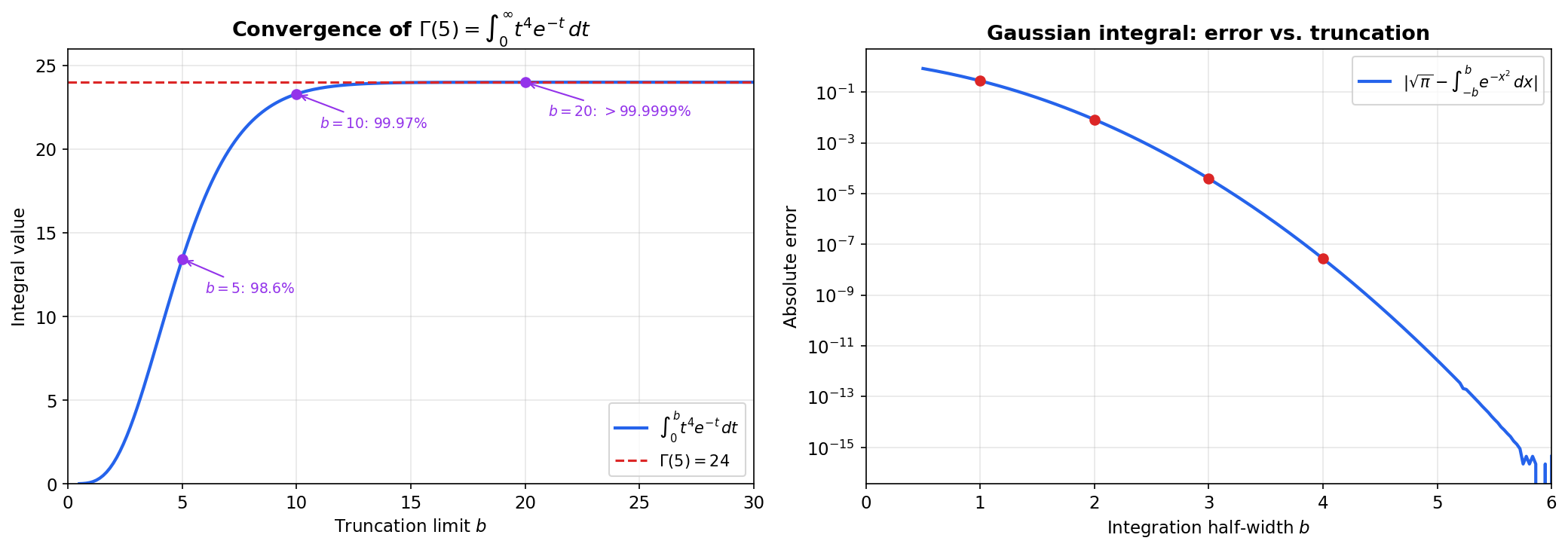
The factorial is defined only for non-negative integers. Is there a smooth function that passes through the points — that is, through — and extends the factorial to all positive real numbers? Euler found one: . This integral converges for , and integration by parts yields , which gives for positive integers.
📐 Definition 4 (The Gamma Function)
For , define
This is a doubly improper integral: the factor may blow up at (a Type II singularity when ), and the integral extends to (Type I).
🔷 Proposition 1 (Convergence of the Gamma Integral)
converges for all .
Near : (since for ), and converges if and only if , i.e., . This is the Type II -test with .
Near : For any , the exponential decay dominates the polynomial growth . Specifically, for large enough, (since for sufficiently large), and converges.
Proof.
Split the integral at : .
For the first piece: on (since ). The integral converges for .
For the second piece: we need as . Since for any (exponential growth dominates polynomial), there exists such that for . Then for , and . The integral is a proper Riemann integral (finite interval, bounded integrand), so it converges trivially.
🔷 Theorem 4 (Gamma Functional Equation)
For : .
Proof.
Integration by parts with and :
The boundary term vanishes at both limits:
- At : (for ).
- At : (exponential decay dominates polynomial growth).
Therefore .
🔷 Theorem 5 (Gamma and the Factorial)
For positive integers : . Also, and .
Proof.
Base case: .
Induction: By the functional equation, , , and generally .
Half-integer value: . Substitute , :
where the last equality is the Gaussian integral (Theorem 7 below).
📝 Example 9 (Half-integer values)
Using the functional equation repeatedly:
In general, . These half-integer Gamma values appear in the surface area of spheres, the volume of balls in , and the normalizing constants of the Student- and Chi-squared distributions.
💡 Remark 5 (The Bohr-Mollerup theorem)
The Gamma function is not just a factorial extension — it’s the factorial extension with the best analytic properties. The Bohr-Mollerup theorem states that is the unique function on satisfying: (i) , (ii) , and (iii) is convex. The log-convexity condition rules out other interpolations like that also satisfy (i) and (ii) but oscillate between the integer values.
The Beta Function
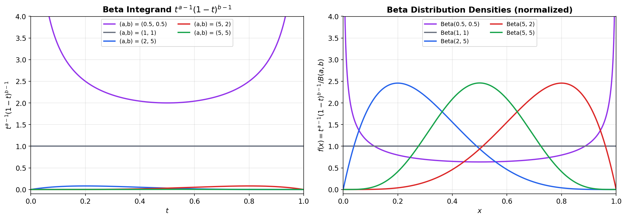
📐 Definition 5 (The Beta Function)
For , define
This is a doubly improper integral when or (Type II singularities at or ). The integral converges for all by the Type II -test at each endpoint: near , the integrand behaves like , and converges iff ; near , it behaves like , and converges iff .
🔷 Theorem 6 (Beta-Gamma Relationship)
For all :
Proof.
Compute the product as a double integral:
Substitute , with and . The Jacobian of this transformation is , so:
Separating:
Therefore , which gives .
(This proof uses Fubini’s theorem and a 2D change of variables — multivariable techniques that will be developed rigorously in Track 4. We preview them here because the result is too important to postpone.)
📝 Example 10 (B(1/2, 1/2) = pi)
Direct verification: . Completing the square and substituting gives .
📝 Example 11 (B(a, 1) and B(1, b))
.
Verify via the Gamma relationship: . Similarly, .
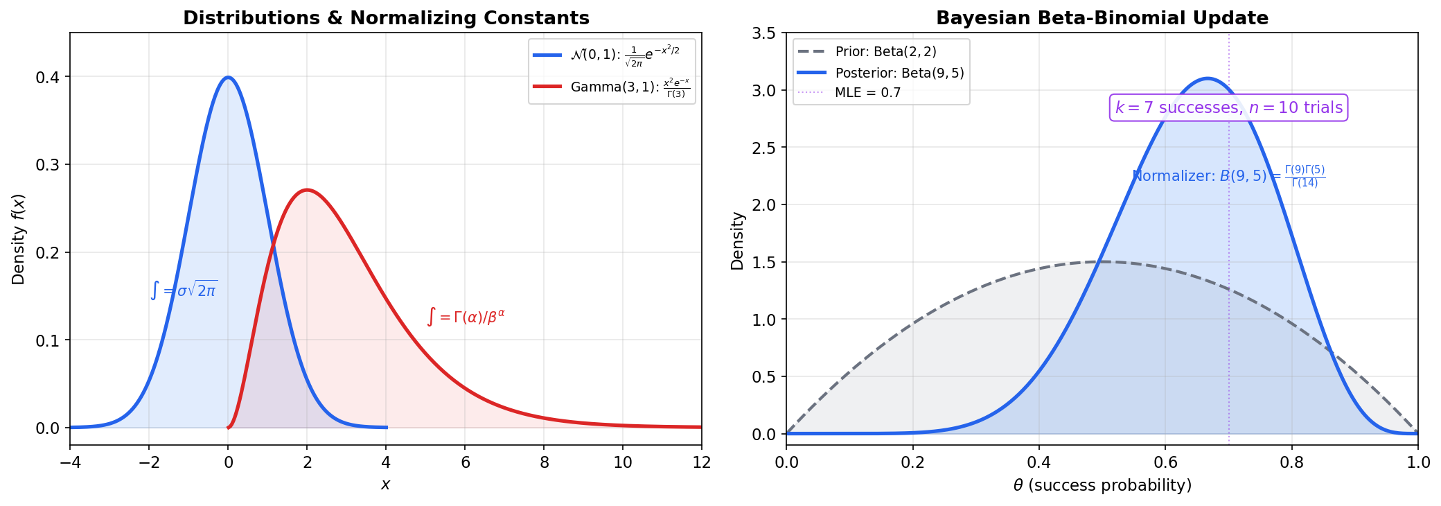
💡 Remark 6 (The Beta distribution)
If , its density is for . The Beta function is precisely the normalizing constant that makes . The parameters control the shape: gives the uniform distribution on ; concentrates the density around ; skews the density toward .
In Bayesian inference, the Beta distribution is the conjugate prior for the Binomial likelihood. If you observe successes in trials and your prior is , the posterior is . The marginal likelihood involves the ratio , which reduces to a ratio of Gamma functions.
The Gaussian Integral
The Gaussian integral is arguably the most important single integral in all of applied mathematics. It normalizes the Gaussian distribution, appears in the definition of , gives the volume of the -sphere, and shows up in quantum mechanics, statistical physics, and signal processing.
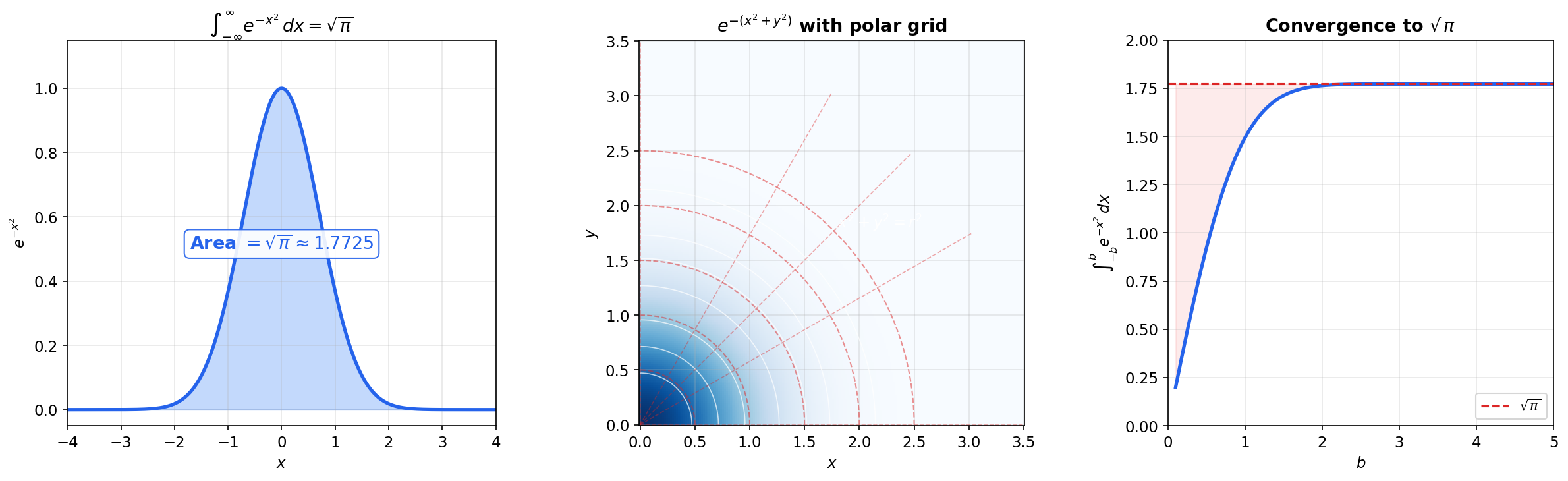
🔷 Theorem 7 (The Gaussian Integral)
Equivalently, .
Proof.
Let . The key trick is to compute as a double integral:
Convert to polar coordinates: , , with Jacobian , and :
The inner integral evaluates by substituting , :
Therefore , so , and .
(This proof uses a double integral and polar coordinates — multivariable tools that will be developed rigorously in Track 4. We preview them here because the result is too important and the proof too elegant to postpone. The reader can follow the geometry: squaring the integral converts a 1D problem into a 2D problem where the radial symmetry of makes the integral tractable.)
🔷 Proposition 2 (Gaussian Integral Variants)
(a) For : . (Substitute .)
(b) Completing the square: .
(c) Even moments: .
These follow from (a) by differentiation with respect to (for the moments) or completing the square in the exponent.
📝 Example 12 (Normalizing the Gaussian density)
The Gaussian density is . We verify :
Substitute , so :
The in the denominator of the Gaussian density is there precisely because — it’s the Gaussian integral doing the normalizing.
💡 Remark 7 (The error function and Gaussian CDF)
The error function is the normalized incomplete Gaussian integral. The Gaussian CDF is:
The error function has no closed-form antiderivative — cannot be integrated in terms of elementary functions. But it can be computed numerically to machine precision by standard libraries (scipy.special.erf, torch.special.erf). The rapid convergence of the Gaussian tail ( for large , known as Mill’s ratio) is what makes sub-Gaussian concentration inequalities so powerful.
Stirling’s Approximation
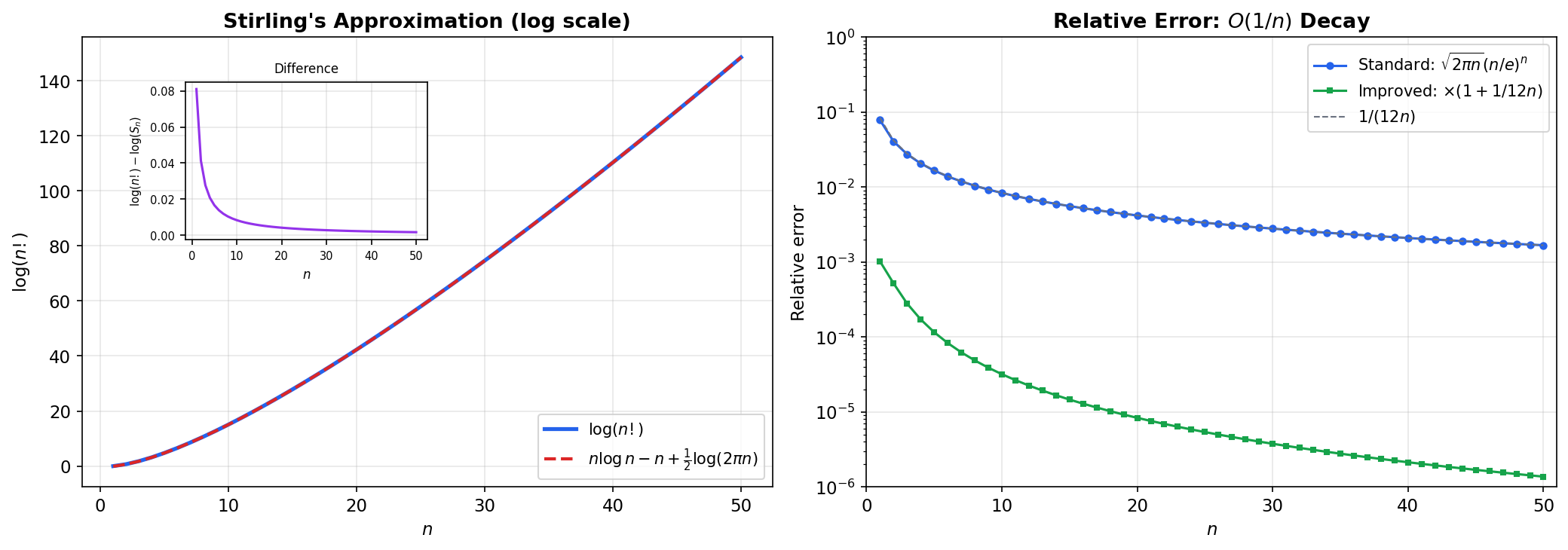
🔷 Theorem 8 (Stirling's Approximation)
More precisely: . The relative error is :
Proof.
We sketch the proof via the Gamma function and Laplace’s method. Write . The integrand has its maximum at (set : gives ).
Substitute to center the integrand at its maximum. Taylor-expanding around :
So for the leading term. Integrating:
The Laplace approximation replaces the integrand by a Gaussian centered at its maximum — the factor is precisely the Gaussian integral. The correction terms (the and higher) come from including the cubic and higher Taylor terms of .
📝 Example 13 (Numerical verification)
| Stirling | Relative error | ||
|---|---|---|---|
| 5 | 120 | 118.02 | 1.65% |
| 10 | 3,628,800 | 3,598,696 | 0.83% |
| 20 | 0.42% | ||
| 50 | 0.17% | ||
| 100 | 0.083% |
The approximation improves as increases — the relative error decreases like .
💡 Remark 8 (Stirling in log form)
In practice, the most useful form is:
This is the form used throughout information theory. The key application: . Applying Stirling to each factorial:
where is the binary entropy function. Stirling’s approximation converts combinatorial counting problems into entropy calculations — this is the foundation of the “method of types” in information theory.
Computational Notes
The special functions from this topic have production-quality numerical implementations in every scientific computing library.
Improper integrals: scipy.integrate.quad handles improper integrals directly — pass np.inf as the upper limit. It uses adaptive Gauss-Kronrod quadrature with automatic singularity detection. For most well-behaved integrands, it achieves machine precision ( relative error).
from scipy.integrate import quad
import numpy as np

# Type I: integral from 1 to infinity of 1/x^2
val, err = quad(lambda x: 1/x**2, 1, np.inf)  # val = 1.0

# Type II: integral from 0 to 1 of 1/sqrt(x)
val, err = quad(lambda x: 1/np.sqrt(x), 0, 1)  # val = 2.0
Special functions: scipy.special provides gamma, beta, erf, and dozens more. For numerical stability, always use scipy.special.gammaln (log-Gamma) instead of computing directly — overflows double precision for , but is representable for much larger .
from scipy.special import gamma, gammaln, beta, erf
import math

gamma(5)      # 24.0 (= 4!)
gammaln(1000) # 5905.22... (log(999!) — doesn't overflow)
beta(2, 3)    # 0.08333... (= 1/12)
erf(1.0)      # 0.8427...
Rule of thumb: Never compute or directly for large . Always work with and exponentiate only at the end, if needed.
Connections to Statistics
Improper integrals are the workhorses of statistical theory: every continuous distribution on an unbounded support is defined via a normalizing improper integral, and tail probabilities, moments, and Bayesian normalizing constants all reduce to such integrals.
Special functions as normalizing constants
The Gamma function normalizes the Gamma, Chi-squared, and Student- distributions. The Beta function normalizes Beta distributions. The Gaussian integral normalizes the Normal. Every continuous distribution on an unbounded support is defined via an improper integral; conjugate priors (Beta-Binomial, Gamma-Poisson, Normal-Normal) are constructed precisely so the posterior normalizer reduces to a ratio of these special functions. See formalStatistics Continuous Distributions and formalStatistics Bayesian Foundations & Prior Selection.
Tail probabilities and large deviations
Tail probabilities are improper integrals. The decay rate (exponential vs. polynomial) determines whether the distribution is sub-Gaussian or heavy-tailed. The Cramér rate function in large-deviation theory controls the exponential rate at which these tail integrals shrink. See formalStatistics Large Deviations.
Moment existence
For heavy-tailed distributions, is an improper-integral convergence question: the moment exists iff the integral converges, which depends on the tail decay rate relative to the power . The Cauchy distribution, with , has no finite mean — a fact that is purely about whether converges. See formalStatistics Expectation & Moments.
Connections to ML
The special functions from this topic are the computational backbone of probability distributions in machine learning. We make the connections explicit.
Normalizing constants for probability distributions
Every probability density satisfies . For the standard parametric families, the normalizing constant is a special function from this topic:
| Distribution | Density kernel | Normalizing constant | Special function |
|---|---|---|---|
| Gaussian integral | |||
| Gamma function | |||
| Beta function | |||
| Gamma function | |||
| (Student) | Gamma function |
Every time you write down a Gaussian, Gamma, or Beta distribution in a model, you’re implicitly using the improper integrals from this topic.
Forward link: Measure-Theoretic Probability on formalML develops the Lebesgue integral framework that makes these normalizing constants rigorous.
Bayesian posterior computation
Conjugate priors are chosen so that reduces to a ratio of special functions:
- Beta-Binomial: Prior , posterior . The marginal likelihood is — a ratio of Beta functions.
- Gamma-Poisson: Prior , posterior . Again, ratios of Gamma functions.
- Normal-Normal: Posterior precision is the sum of prior and likelihood precisions. The normalizing constant involves .
When conjugacy is unavailable, these integrals must be computed numerically via MCMC or variational inference.
Forward link: Bayesian Nonparametrics on formalML develops the general Bayesian inference framework.
Stirling’s approximation in information theory
The entropy of the binomial distribution is:
via Stirling applied to . The “method of types” uses to count the number of binary strings with a given empirical frequency. Stirling converts combinatorial counting into entropy maximization.
Forward link: Shannon Entropy on formalML develops the full information-theoretic framework.
Tail probabilities and concentration
The tail probability is an improper integral. For a standard Gaussian:
(Mill’s ratio bound). The tail decay rate determines whether the distribution is sub-Gaussian, sub-exponential, or heavy-tailed, and thereby governs the strength of available concentration inequalities.
Forward link: Concentration Inequalities on formalML develops sub-Gaussian and sub-exponential tail bounds.
Connections & Further Reading
Prerequisites — topics you need first
The Riemann Integral & FTC
The Riemann integral defined on bounded functions on bounded intervals is the starting point. Improper integrals extend this via limits: ∫₁∞ f = lim_{b→∞} ∫₁ᵇ f. The FTC, linearity, monotonicity, and comparison properties of the integral are used throughout.
Mean Value Theorem & Taylor Expansion
Taylor expansion near singularities determines the convergence behavior of Type II improper integrals. Stirling’s approximation uses the method of Laplace (a saddle-point approximation that is essentially a second-order Taylor expansion of the log-integrand). The limit comparison test relies on the asymptotic analysis tools from Topic 6.
Sequences, Limits & Convergence
Improper integrals are defined as limits of proper integrals. The convergence/divergence analysis parallels the convergence theory of sequences from Topic 1, and the comparison test for improper integrals is the continuous analog of the comparison test for sequences.
Completeness & Compactness
The Monotone Convergence principle for sequences (a consequence of completeness, Topic 3) justifies the existence of limits defining convergent improper integrals: if the truncated integrals form a bounded, monotone sequence, the limit exists.
The Derivative & Chain Rule
The Gamma function’s functional equation Γ(s+1) = sΓ(s) is proved via integration by parts (the product rule in reverse, Topic 5/Topic 7). Differentiation under the integral sign — differentiating ∫ f(x,t) dt with respect to a parameter — uses the derivative theory from Topic 5.
Where this leads — next in formalCalculus
On to formalStatistics — where this calculus powers inference
Continuous Distributions
The Gamma function Γ(s) = ∫₀^∞ t^(s-1) e^(-t) dt normalizes the Gamma, Chi-squared, and Student-t distributions. The Beta function normalizes Beta distributions. The Gaussian integral ∫ e^(-x²) dx = √π normalizes the Normal. Every continuous distribution on unbounded support is defined via an improper integral.
Bayesian Foundations And Prior Selection
Conjugate priors (Beta-Binomial, Gamma-Poisson, Normal-Normal) are constructed so the posterior normalizer reduces to a ratio of Gamma or Beta functions. Improper priors (Jeffreys, flat) require the improper-integral machinery to verify posterior propriety.
Large Deviations
Tail probabilities P(X > t) = ∫_t^∞ f(x) dx are improper integrals. The rate-function asymptotics in Cramér's theorem control the exponential decay of these tail integrals.
Expectation Moments
Moment existence for heavy-tailed distributions is an improper-integral convergence question: E[X^k] = ∫ x^k f(x) dx exists iff the integral converges, which depends on the tail decay rate relative to the power k.
On to formalML — where this calculus powers ML
Measure Theoretic Probability
Every probability density satisfies ∫ f(x) dx = 1, an improper integral. The Gamma and Beta functions are normalizing constants for the Gamma, Chi-squared, Beta, and Dirichlet distributions. The transition from improper Riemann integrals to Lebesgue integrals resolves convergence issues with conditional integrals and enables measure-theoretic probability.
Bayesian Nonparametrics
Bayesian posteriors require ∫ likelihood × prior dθ over unbounded parameter spaces. Conjugate priors (Gamma-Poisson, Beta-Binomial, Normal-Normal) are designed so these improper integrals reduce to ratios of Gamma and Beta functions, yielding closed-form posteriors.
Shannon Entropy
Differential entropy h(X) = -∫ f(x) log f(x) dx and KL divergence are improper integrals over ℝ. For the Gaussian, this evaluates to ½ log(2πeσ²) via the Gaussian integral. Stirling’s approximation gives the entropy of the binomial distribution: H(Bin(n,p)) ≈ ½ log(2πnp(1-p)).
Concentration Inequalities
Tail bounds P(X > t) = ∫ᵗ∞ f(x) dx are improper integrals. The decay rate (exponential vs. polynomial tails) determines sub-Gaussian vs. heavy-tailed behavior. Stirling’s approximation appears in sharp bounds for binomial tails via the entropy method.
References
- book Abbott (2015). Understanding Analysis Chapter 7.4 covers improper integrals as an extension of the Riemann integral — our primary reference for the convergence theory and comparison tests
- book Rudin (1976). Principles of Mathematical Analysis Chapter 8 develops special functions including the Gamma function with characteristic concision — useful for the functional equation and Stirling’s approximation
- book Spivak (2008). Calculus Chapter 18 on improper integrals with geometric motivation, and Chapter 19 on the Gamma function — the best reference for combining rigor with intuition
- book Graham, Knuth & Patashnik (1994). Concrete Mathematics Chapter 9 develops Stirling’s approximation with detailed asymptotics — the most thorough treatment of the factorial’s asymptotic behavior
- book Folland (1999). Real Analysis Chapter 2 on the Lebesgue integral — useful for understanding where improper Riemann integration fails and why the Lebesgue framework handles these issues naturally
- book Bishop (2006). Pattern Recognition and Machine Learning Appendix B collects the special function identities (Gamma, Beta, Gaussian) used throughout Bayesian ML — the ML practitioner’s reference for these functions