Probability & The Union Bound
Kolmogorov axioms, the inequality every multiple-testing and generalization proof leans on, and the ladder from Markov to Hoeffding that turns one event into many.
Abstract. Probability is the first place every machine learning and statistics argument lands. This topic builds the apparatus that almost every such argument uses: a small set of axioms (Kolmogorov), a single combinatorial bound (Boole / the union bound), and a ladder of three increasingly sharp tail inequalities (Markov, Chebyshev, Hoeffding). The union bound is the inequality that turns "one bad event has small probability" into "none of these m bad events happens, with high probability." It is the entire engine behind Bonferroni's family-wise error rate control in multiple testing, behind PAC generalization bounds over a hypothesis class, behind UCB confidence sets in bandit algorithms, and behind the first Borel–Cantelli lemma. We prove every inequality fully, derive Hoeffding's bound from the moment generating function and Markov's inequality, and finish with the "union bound + concentration" pattern that every modern learning-theory result relies on. No measure theory is required — the topic is the on-ramp to the rigorous probability that the Measure & Integration track will provide.
1. Three Puzzles the Union Bound Solves
We open with three apparently unrelated questions. By the end of the topic each will be a one-line application of a single inequality.
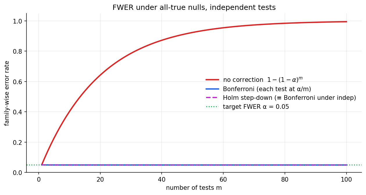
Puzzle 1 — Why does the Bonferroni correction work? A researcher runs hypothesis tests, each at significance level . Under the null hypothesis that all effects are zero, what is the probability that at least one test falsely rejects? If the tests were independent, the answer would be — almost certain. The Bonferroni correction says: test each hypothesis at level instead. Then no matter what the dependence between the tests is, the family-wise error rate is at most . The proof, when we get to it, is one line. It is the union bound.
Puzzle 2 — What does “infinitely often” even mean? Toss a fair coin forever. The event “heads occurs infinitely often” is intuitive but slippery: it is a statement about the entire infinite tail of the sequence, not about any finite prefix. The Borel–Cantelli lemmas give it a precise set-theoretic form and a sharp probabilistic dichotomy: if , then occurs infinitely often with probability ; if and the are independent, then occurs infinitely often with probability . The first half of that dichotomy is — again — a corollary of the union bound.
Puzzle 3 — Why does a learning algorithm generalize? A machine-learning system picks the best hypothesis from a finite class by minimizing the training error over samples. We want a bound on the true risk — the error on fresh data. For any single fixed hypothesis , Hoeffding’s inequality gives . But is not a single fixed hypothesis — it is whichever member of happens to win the training-error contest. So we need a bound that holds uniformly over . The PAC generalization bound delivers exactly that:
The inequality on the left is upgraded to one on the right by paying a factor of — a price that, on the log scale of the deviation, is only . The mechanism is the union bound, again.
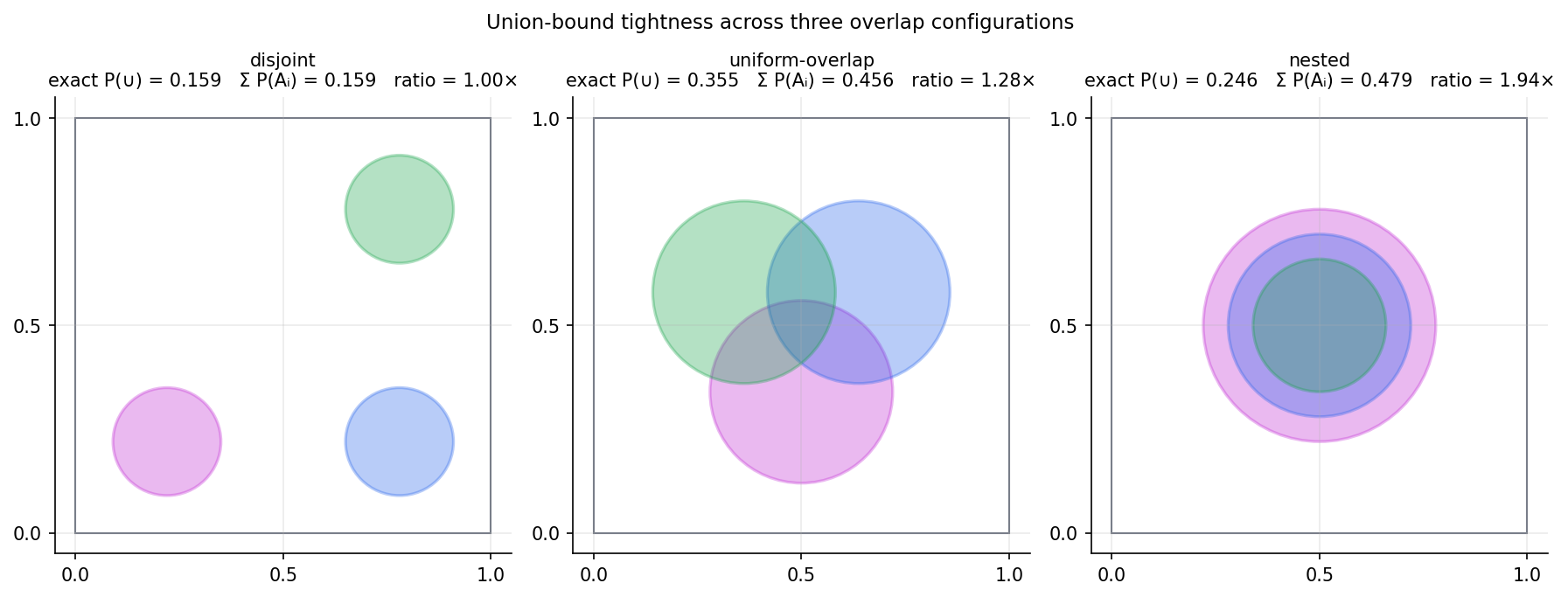
Three puzzles, three subjects, one inequality. The interactive below previews the geometry. Drag the events apart and the union bound becomes tight; drag them together and the gap opens.
- Tightness ratio
- 1.29×
- Gap Σ − exact
- 0.102
- Bonferroni-2 closer?
- yes (by 0.114)
The blue bar is the exact P(⋃ Aᵢ). The red bar is the union-bound estimate Σ P(Aᵢ). When the events are disjoint, the two bars coincide (ratio = 1). When the events overlap, Σ P(Aᵢ) overshoots and the gap measures the looseness.
The editorial pivot of this topic. Everything you have done in formalCalculus so far has been about functions on the real line: limits, derivatives, integrals, series of numbers. Probability is about subsets of an abstract sample space, and the operations are union, intersection, and complement instead of addition, multiplication, and composition. The vocabulary is different, but the analytic moves are the same — limits of sequences, convergence of sums, exchange of supremum and limit. In Sigma-Algebras & Measures, the measure-theoretic foundations make this analogy exact. For now we proceed at the elementary level: probabilities are non-negative numbers attached to subsets of a sample space, they sum to one, and the only inequalities we need are short combinatorial arguments.
2. The Kolmogorov Axioms
A probability is a function that takes events (subsets of a sample space) and returns numbers in , subject to three axioms. The axioms are short; their consequences are everything.
📐 Definition 1 (Probability space)
A probability space is a triple where:
- is a non-empty set, the sample space — the set of all possible outcomes.
- is a collection of subsets of , the events — sets to which we are willing to assign a probability. We require , whenever , and whenever each (closure under countable unions).
- is a function satisfying three axioms:
- (K1) Non-negativity. for every .
- (K2) Normalization. .
- (K3) Countable additivity. For any disjoint sequence of events, .
💡 Remark 1 (Events without sigma-algebras)
The closure conditions on make it a sigma-algebra. Why bother — why not let every subset be an event? For finite or countable , the answer is: we can let every subset be an event, by taking . The condition is automatically satisfied and the question never arises. For uncountable — like with the “length” probability — there exist subsets to which no consistent probability can be assigned, and has to be smaller than . That non-trivial story is told in Sigma-Algebras & Measures (forward). For this topic, take to be “the subsets we know how to measure” and proceed.
The axioms are sparse, but they force every standard probability identity. We collect the most-used consequences before moving on.
🔷 Proposition 1 (Immediate consequences of the axioms)
Let be a probability space. Then:
- .
- for every .
- Monotonicity: if , then .
- Finite additivity: for disjoint events , .
- Continuity from below: if is an increasing sequence of events, then .
Proof.
(1) Take for all in (K3). The events are disjoint, so . If then the right-hand side is , contradicting . So .
(2) disjointly, so by (K3) applied to the finite sequence and (1), .
(3) Write disjointly. By (K3) (or by (4) applied to a 2-element disjoint family), since by (K1).
(4) Pad the finite disjoint sequence with empty sets: . Apply (K3) and use (1) to discard the empty-set terms.
(5) Set and for . The are pairwise disjoint, (since the chain is increasing), and for every . By (K3) and (4):
The convergence of the limit on the right is automatic — partial sums of a non-negative series are monotone increasing and bounded by , so they converge.
Three examples anchor the axioms in concrete computations.
📝 Example 1 (The fair die)
Let , , for each . By finite additivity, the probability of any event is the sum of the per-outcome probabilities of its members. For instance, , and . The axioms reduce to “count and divide.”
📝 Example 2 (A countable, non-uniform sample space)
Let and define . Since , this defines a probability measure on by countable additivity: for every . This is the “geometric trials” model — the probability of needing exactly trials until the first success, when each trial is a fair coin. The sample space is countably infinite; the axioms still apply unchanged.
📝 Example 3 (Continuous uniform on [0, 1] (informal))
Let and define for . This is the “uniform random number” model. To say which subsets of are in in full generality requires the measure-theoretic machinery of Sigma-Algebras & Measures (forward). For this topic, take on intervals as an oracle and proceed; no construction in the body of this topic depends on which specific subsets of are measurable.
💡 Remark 2 (Why countable, not finite)
Why does (K3) ask for countable additivity rather than just finite additivity? Because the most important consequences — continuity from below (Proposition 1(v)), the first Borel–Cantelli lemma (Theorem 3), and the convergence of partial-sum probabilities — all require taking limits of an infinite sequence of disjoint events. A theory built on finite additivity alone cannot say “the probability that heads occurs infinitely often is zero” — that statement is about an infinite intersection of unions, and finite additivity gives no access to the limit. The price of countable additivity is the sigma-algebra constraint on ; the reward is the entire analytic machinery of the rest of this topic.
3. Conditional Probability and Independence
Conditioning is how probability talks about evidence. The formula is one division.
📐 Definition 2 (Conditional probability)
For events with , the conditional probability of given is
💡 Remark 3 (What conditioning does)
Conditioning on rescales the universe to the part of where occurred. Three things follow immediately: (i) , so is normalized; (ii) for every , so it is non-negative; (iii) countable additivity of follows from countable additivity of applied to the numerator. So is itself a probability measure on — a fact we will use without further comment.
🔷 Proposition 2 (Multiplication rule)
For events with ,
🔷 Proposition 3 (Law of total probability)
If is a finite or countable partition of (the are pairwise disjoint and ) with each , then for any event :
🔷 Proposition 4 (Bayes' rule)
For events with :
Combined with the law of total probability (when the denominator is unknown), for any partition with :
Bayes’ rule is a corollary, not a headline. It says: to invert a conditional, multiply by the marginal of the new conditioner and divide by the marginal of the old. Every proof is the same line — , divide.
Independence is the structural property that makes joint probabilities factor.
📐 Definition 3 (Independence (pair, family))
- Events and are independent if .
- A family is mutually independent (or simply independent) if for every finite subset ,
- A family is pairwise independent if every pair of events in the family is independent.
Mutual independence is strictly stronger than pairwise independence. The standard counterexample uses three events constructed from two fair coin tosses.
📝 Example 4 (Pairwise but not mutually independent — the 3-coin example)
Take — four outcomes, each with probability . Let be the event “the -th coordinate equals .” Then for each (two of the four outcomes have a in position ).
For any , exactly one of the four outcomes has s in both positions, so . Every pair is independent.
But would require an outcome with s in all three positions — and there is no such outcome in . So , while . The three events are pairwise independent but not mutually independent.
The structural reason: the third coordinate of each outcome equals the parity (XOR) of the first two. Knowing any one coordinate tells you nothing about another; knowing any two determines the third. Independence is a family-level property, not a sum of pairwise properties.
💡 Remark 4 (Independence is a probability statement, not a logical one)
Two events and are independent under one probability measure and dependent under another, even when the underlying sets are the same. Independence is a property of the triple , not of the events alone. In statistical practice this means independence is an assumption that needs justification, not a logical certainty — two events about completely different physical systems can still be statistically dependent if the data-generating distribution links them.
4. The Union Bound (Boole’s Inequality)
The centerpiece of this topic. The statement is one line; the proof is two; the consequences fill the rest of the curriculum.
🔷 Theorem 1 (Boole's inequality (the union bound))
For any countable sequence of events in a probability space:
Equality holds if and only if the events are pairwise disjoint up to a null set — i.e., for every .
Proof.
Define a disjointified sequence: set , and for let . Three properties hold by construction.
First, the are pairwise disjoint: if , then , so contains no point of .
Second, for every (subtracting a set can only make smaller).
Third, . The direction is immediate from . For the direction: any lies in some ; let be the smallest index with . Then but for , so .
Now apply countable additivity to and monotonicity to :
For the equality case: by Proposition 1(iv) applied to the disjoint union . So forces every , which is equivalent to every pairwise intersection for .
The proof is the bookkeeping of disjointifying a sequence — the entire content is that “the events overlap” subtracts from the total. The next two consequences are the working tools.
🔷 Corollary 1 (Bonferroni's inequality)
For any finite or countable family of events :
Proof.
By De Morgan, . So
where the inequality is Boole applied to the complements.
📝 Example 5 (Bonferroni and multiple testing)
This is the canonical application of Corollary 1, and Puzzle 1 of §1 resolved. Suppose we run statistical tests; let be the event “test falsely rejects the null hypothesis.” If each test is run at level — that is, under the null — then by Boole on the complements,
Choosing guarantees the family-wise error rate is at most , regardless of the dependence between the tests. The price is power: each individual test is run at a much stricter level than , so the test loses sensitivity. This is the trade-off every multiple-testing correction faces, and Bonferroni is the simplest possible solution. See Multiple Testing and False Discovery → formalStatistics for sharper procedures (Holm step-down, Hochberg, Benjamini–Hochberg FDR control) that all begin from this same union-bound observation.
📝 Example 6 (The uniform tail-bound pattern)
This pattern will appear repeatedly. Let be random variables — possibly dependent in complicated ways — and suppose each satisfies the same per-variable tail bound . Then by Boole,
To control the maximum at confidence , choose so that — equivalently, . For the Hoeffding tail that we will prove in §8, this gives — the classical price of taking a union over events.
The pattern is so general that, in machine-learning practice, “apply a union bound” is almost always shorthand for this single move: per-event exponential tail, events, pay a tax in the deviation.
📝 Example 7 (A loose bound is still informative)
Take fair, independent coins; let be the event “coin lands heads.” The exact probability of at least one head is . The union bound gives
which is useless — it exceeds , the absolute upper bound on any probability. The union bound is tight when events are nearly disjoint and uninformative when events are highly overlapping. Drag the circles in the flagship visualization together to see the bound’s ratio blow up; drag them apart to see the bound recover to exactness.
Loose bounds are not failures. They are advertisements for a different tool — usually inclusion–exclusion (§5) or a structural argument that exploits the overlap. The union bound’s value is not its sharpness but its generality: it asks nothing about how the events relate.
💡 Remark 5 (Boole vs. Bonferroni vs. inclusion–exclusion)
Three closely-related results live in this chapter. Boole’s inequality (Theorem 1) is a one-sided upper bound on . Bonferroni’s inequality (Corollary 1) is the lower bound on that falls out of Boole on the complements. Inclusion–exclusion (Theorem 2 below) is an exact equality. The reason to reach for Boole instead of inclusion–exclusion in a proof is that Boole needs nothing about pairwise or higher-order intersections — only the marginal . This is exactly what makes Boole the workhorse of high-dimensional and distribution-free arguments: in those settings, joint probabilities of events are typically unknown or uncomputable, but marginals are not.
5. Inclusion–Exclusion
When the marginals are not enough — when the overlaps are computable and we want an exact probability — inclusion–exclusion is the tool.
🔷 Theorem 2 (Inclusion–exclusion (finite version))
For any finite family of events :
Proof.
Proof sketch by induction on . The base case is
which follows from disjointly and .
For the inductive step, suppose the formula holds for events. Write
apply the case to the two events and :
The induction hypothesis applies twice — to the first term (an -fold union) and to the third term (the union of the intersections , also an -fold union of events). Expand both, collect terms by intersection cardinality, and verify that the signs and coefficients combine to give the claimed formula. The algebra is mechanical and is performed in full in the companion notebook.
The 3-event case is worth writing out explicitly — it is the formula most often used by hand.
📝 Example 8 (The 3-event case)
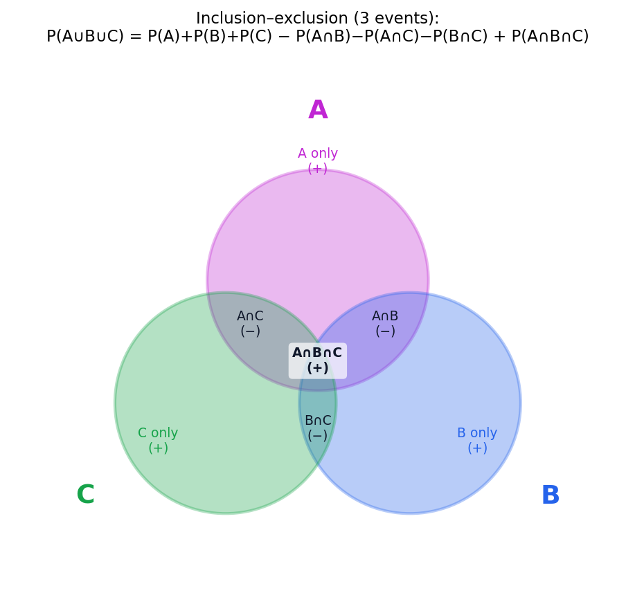
For events :
Verification on the uniform model over . Let with each outcome having probability , and let be the event “the -th coordinate is .” Then , for , and . The right-hand side is , which matches . The accompanying notebook reproduces this and the 4-event and 5-event cases for sanity.
📝 Example 9 (Derangements via inclusion–exclusion)
A derangement is a permutation with no fixed points. The probability that a uniformly random permutation of is a derangement equals
The proof is inclusion–exclusion in three lines. Let be the event ” is a fixed point.” Then — once is fixed, the remaining positions can be permuted in ways. More generally, for any distinct indices, and there are such -subsets. Inclusion–exclusion gives
Subtracting from gives the derangement probability , which is the partial-sum approximation to .
This is a classical combinatorial identity, but it is also a sanity check for the analytic side: by Series Convergence & Tests the alternating series converges absolutely to , and the rate of convergence is faster than geometric — even at the derangement probability is correct to four decimal places.
💡 Remark 6 (Bonferroni's inequalities — the full hierarchy)
Boole’s inequality is the first member of a hierarchy. Truncating the inclusion–exclusion alternating sum at an even number of terms gives an upper bound on ; truncating at an odd number gives a lower bound. The first odd truncation — a single term, — is exactly Boole. The next two truncations are
(The lower bound is the “Bonferroni depth-2” bar in the flagship visualization.) The full hierarchy — Bonferroni’s inequalities — provides arbitrarily tight bounds at the cost of summing joint probabilities at depth . In practice we rarely go past depth 2, because the gain in tightness beyond that is small relative to the explosion of joint terms.
6. The Borel–Cantelli Lemmas
Boole’s inequality is the engine; the Borel–Cantelli lemmas are its first major application. They convert a question about the infinite tail of a sequence of events — does the event occur infinitely often? — into a question about a series of probabilities . The two halves of the dichotomy are mirror images of one another: one is union-bound short, the other uses the inequality and independence.
📐 Definition 4 (The 'infinitely often' event)
For a sequence of events , the event ” occurs infinitely often” is
Its complement is the event ” occurs only finitely many times”:
💡 Remark 7 (Set-theoretic limsup, revisited)
The definition is the set-theoretic limsup the reader saw in Sequences, Limits & Convergence translated into events. A point is in precisely when belongs to infinitely many of the . The “for every there exists ” structure of the definition is exactly the standard unwinding of “infinitely often.”
The complementation rule — a countable De Morgan — is used in the proof of the second Borel–Cantelli lemma. Verify by chasing definitions:
🔷 Theorem 3 (First Borel–Cantelli lemma)
If , then
Proof.
By monotonicity of and Boole’s inequality, for every :
Since , the tail of the series satisfies as — this is the definition of convergence of a series of non-negative terms (see Series Convergence & Tests).
Now is a decreasing intersection: as grows, fewer terms are in the union, so shrinks. By continuity of probability (Proposition 1(v) applied to complements, or its mirror image for decreasing sequences):
Since probabilities are non-negative, .
🔷 Theorem 4 (Second Borel–Cantelli lemma)
If the events are mutually independent and , then
Proof.
It suffices to show that for every , because then by countable subadditivity (Boole) on the union , the event has probability and its complement has probability .
Fix and any finite truncation . By mutual independence of the ‘s, the events are also mutually independent (the complement of an independent event is independent of the original family). So
Use the inequality for on each factor:
Now let . The partial sum diverges to (because the full series does, and the partial sum from onward differs from the full sum by a finite quantity). So the exponential tends to :
The first equality uses continuity of probability for decreasing intersections (Proposition 1(v) applied to complements). Since probabilities are non-negative, .
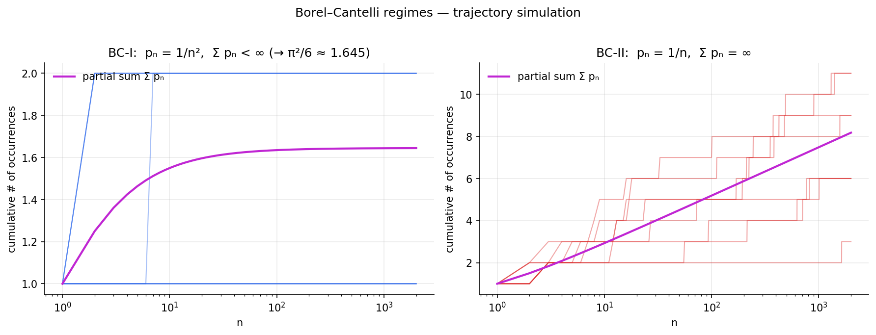
The two lemmas are not symmetric. The first uses only countable subadditivity and the convergence of a series — no independence. The second requires independence (or some substitute, like pairwise independence with a Kolmogorov-style covariance bound), and the inequality does the work that would do asymptotically. Two examples make the transition between the two regimes concrete.
📝 Example 10 (The harmonic-versus-quadratic threshold)
Take independent events with . The series converges iff (the -series test from Series Convergence & Tests). So:
- : BC-I applies, . The events stop occurring after some finite point with probability one.
- : BC-II applies, . The events recur forever.
The threshold is exactly at — the harmonic series. The accompanying interactive visualization sweeps across the threshold and shows the cumulative-indicator trajectories diverging or stabilizing in real time.
📝 Example 11 (Independence cannot be dropped from BC-II)
Take all events equal: for every , with . The events are not independent — they are perfectly dependent — and trivially. But
which is not in general. Independence is what makes the BC-II conclusion robust: under independence, the divergent sum forces the product to ; without it, the joint probabilities can conspire to keep the all-fail event positive.
There are partial substitutes — pairwise independence plus a Kolmogorov bound on covariances, exchangeability, etc. — but they are downstream of the full machinery of conditional expectation, and we defer them to Sigma-Algebras & Measures (forward) and to formalStatistics’s hypothesis-testing topic.
The viz below lets you toggle between (BC-II divergent) and (BC-I convergent), and watch the trajectories diverge or stabilize. The power-law slider sweeps across the threshold at .
- ∑_{k ≤ N} p_k
- 1.643
- mean indicator-sum @ N
- 1.88
- max indicator-sum @ N
- 4
When ∑ p_n is bounded (BC-I), trajectories stabilize — the indicator-sum stops growing. When ∑ p_n diverges and the events are independent (BC-II), trajectories grow without bound, tracking the partial-sum curve in expectation.
💡 Remark 8 (Toward Kolmogorov's 0–1 law)
The Borel–Cantelli lemmas are special cases of a deeper structural fact: any tail event of an independent sequence — an event in the σ-algebra generated by for every — has probability or . The event is a tail event by construction. Kolmogorov’s 0–1 law extends this to any tail event of an independent sequence, including the event “the Strong Law of Large Numbers holds for this sequence” (i.e., ). The full statement and proof require the measure-theoretic σ-algebra apparatus of Sigma-Algebras & Measures (forward) and is the entry point to the Strong Law and the law of the iterated logarithm.
7. Markov’s and Chebyshev’s Inequalities
The Borel–Cantelli lemmas convert “probability of an asymptotic event” into “convergence of a series.” We now turn to the other half of the picture: bounding — the probability that a single random variable exceeds a threshold — by an expectation. The first two rungs of the concentration ladder are short and useful; both are direct corollaries of the axioms.
🔷 Theorem 5 (Markov's inequality)
Let be a non-negative random variable with finite expectation , and let . Then
Proof.
For and , observe the pointwise inequality
To see it: on the event , the indicator is , so the left-hand side is , and by hypothesis; on the complement, the indicator is , so the left-hand side is , and since . Taking expectations of both sides (using linearity and monotonicity of expectation),
Divide by .
Markov is a one-line inequality whose strength is its lack of assumptions: no second moment, no boundedness, no independence — just non-negativity and a finite mean. The price is looseness: a bound polynomial in rather than exponential. The geometric reading sharpens the intuition.
💡 Remark 9 (Geometric reading of Markov)
For non-negative , the tail-integral identity from Improper Integrals & Special Functions
says the area under the survival curve equals the mean. Markov’s inequality says that no rectangle inscribed under the survival curve can have area greater than the total area:
The rectangle in question has width and height , and it fits under the survival curve because the survival function is non-increasing.
![Survival curve P(X > t) for an Exp(1) random variable, with the Markov rectangle of width a and height P(X ≥ a) shaded under the curve. The rectangle's area cannot exceed the total area, which equals E[X].](/images/topics/probability-and-union-bound/markov-geometric.png)
Chebyshev’s inequality is the next rung. It is not a new technique — it is Markov applied to a particular transformation of .
🔷 Theorem 6 (Chebyshev's inequality)
Let be a random variable with and finite variance . Then for any :
Proof.
Apply Markov’s inequality to the non-negative random variable at the threshold :
But . So .
Chebyshev gives a polynomial tail rather than the constant of Markov — a strict improvement whenever is large enough that the squaring helps. It is also distribution-free: any random variable with finite variance gets the same bound. The single most important application is the Weak Law of Large Numbers.
📝 Example 12 (Chebyshev gives a 1/n rate (Weak Law of Large Numbers))
Let be independent and identically distributed with mean and finite variance . Let be the sample mean. By the linearity of expectation and the variance of an independent sum,
Chebyshev applied to gives, for any :
As , the right-hand side tends to , so in probability. This is the Weak Law of Large Numbers, derived from one inequality. The rate is polynomial in : doubling halves the bound.
Hoeffding’s inequality (Theorem 7 below) replaces this polynomial rate with an exponential one when the are bounded — a strict improvement for moderate-to-large deviations.
💡 Remark 10 (Why Chebyshev is loose for sub-Gaussian tails)
For a Gaussian random variable , the actual tail is — exponentially decaying. Chebyshev gives only — polynomial. At , the Gaussian tail is , while Chebyshev says — off by nearly two orders of magnitude.
This gap between polynomial Chebyshev bounds and exponential true tails is what motivates Hoeffding’s inequality: when we know more about the random variable (boundedness, sub-Gaussian moment generating function), we can replace the polynomial decay with an exponential one. The MGF method developed in §8 is the standard route.
8. Hoeffding’s Inequality
The third rung of the concentration ladder. Hoeffding’s inequality replaces Chebyshev’s polynomial decay with an exponential decay, at the cost of one additional hypothesis: that the random variables are bounded. The proof is the canonical moment-generating-function method of concentration, and it is short.
📐 Definition 5 (Moment generating function)
For a random variable , the moment generating function (MGF) is
defined for those at which the expectation is finite.
💡 Remark 11 (MGF as a self-contained tool)
This is the only place in the topic where the MGF appears. We use it as a single technical device: has a small MGF has light tails. Markov’s inequality applied to the non-negative random variable converts a bound on the MGF into a bound on . The rigorous Lebesgue-integral foundations of expectation, conditions for the MGF to exist in a neighborhood of , and the Cramér–Chernoff method are developed in The Lebesgue Integral (forward) and in formalML’s Concentration Inequalities → formalML. Here we treat the MGF as a black box that produces the bound.
The technical heart of the proof is the following lemma, which bounds the MGF of a centered bounded random variable by a Gaussian-like envelope.
🔶 Lemma 1 (Hoeffding's lemma)
If is a random variable with and almost surely, then for every :
Proof.
Proof sketch. The function is convex. For , convexity gives the chord bound
Take expectations on both sides, using :
where is the logarithm of the right-hand side. Direct calculus shows , , and uniformly in . By Taylor’s theorem (see Taylor Series and Polynomial Approximation),
Exponentiating gives the claim. The full algebra is performed in the companion notebook.
With Hoeffding’s lemma in hand, the proof of Hoeffding’s inequality is a clean application of Markov, independence, and a one-variable optimization.
🔷 Theorem 7 (Hoeffding's inequality)
Let be independent random variables with almost surely. Let . Then for any :
The symmetric two-sided form follows by union bound on the two one-sided events:
Proof.
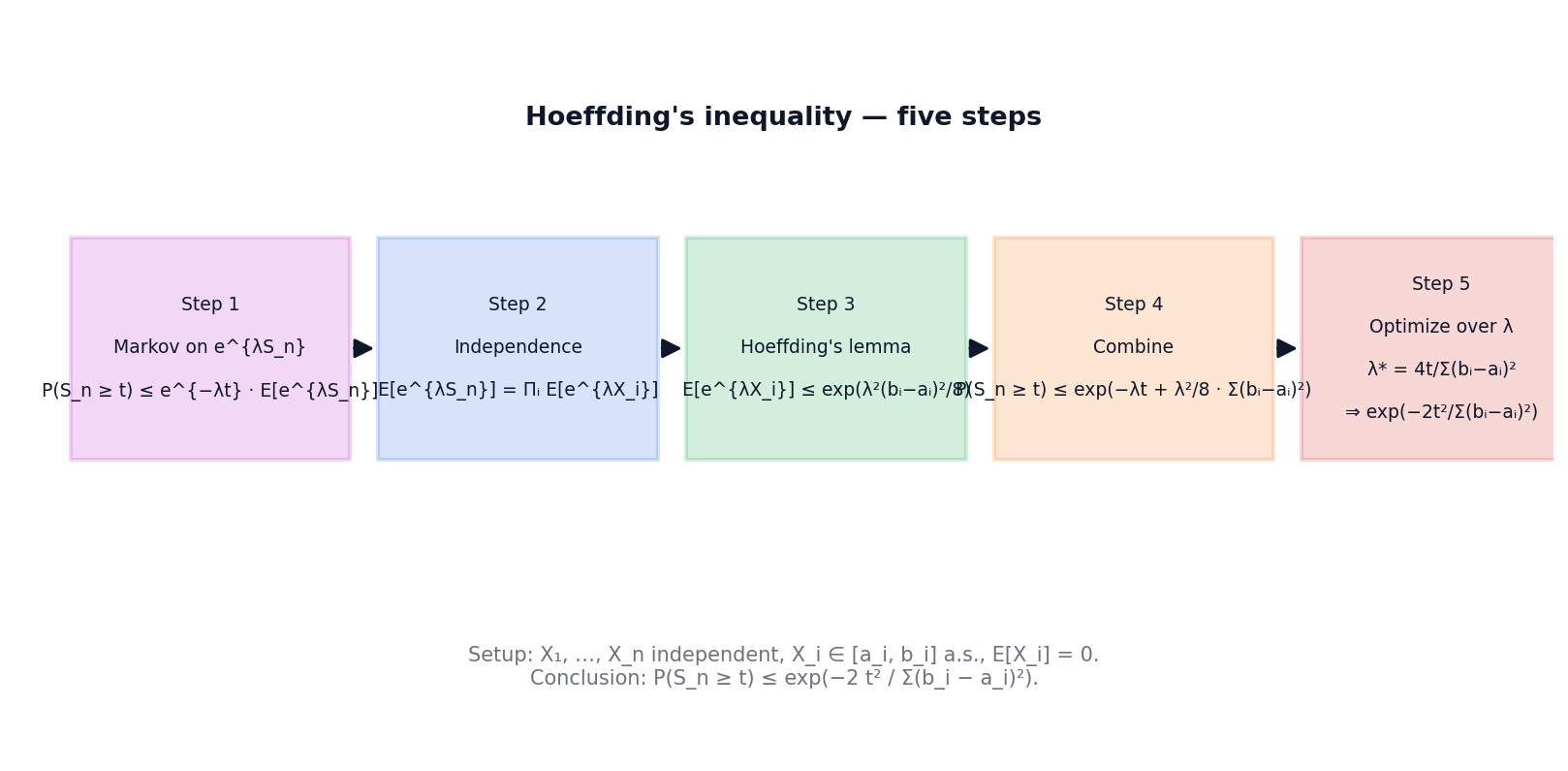
Full proof. Without loss of generality assume each (otherwise subtract the means; the bound is unchanged). The proof proceeds in five steps, each rendered as its own display block to keep the KaTeX-renderable structure clean.
Step 1. Apply Markov’s inequality to the non-negative random variable at the threshold (for any ):
Step 2. By independence of the , the MGF of factors:
Step 3. Apply Hoeffding’s lemma to each (centered, bounded in ):
Multiply across to obtain .
Step 4. Combine Steps 1 and 3:
Step 5. The right-hand side is a quadratic in ; its minimum over is at . Substituting back:
This is the one-sided bound. The two-sided bound follows by applying the same argument to (which gives ) and combining the two one-sided events via Boole’s inequality, contributing the factor of .
The most common form in practice is the i.i.d. average over -bounded variables.
🔷 Corollary 2 (Hoeffding for i.i.d. averages on [0, 1])
Let be i.i.d. with , and let . Then for any :
Proof.
Apply Theorem 7 to with for every and . The denominator , so the exponent becomes .
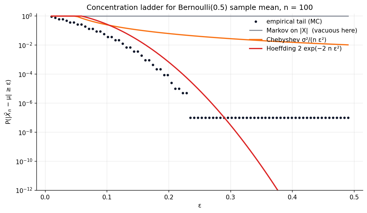
📝 Example 13 (Hoeffding vs. Chebyshev on Bernoulli sums)
Let be i.i.d. Bernoulli, . The variance of is , so by Chebyshev, . By Hoeffding (Corollary 2 applied to with ), the same tail is at most .
At standard deviations: Chebyshev gives , Hoeffding gives . Hoeffding is six orders of magnitude tighter at three sigmas. At , the gap is . The accompanying visualization plots all three bounds against the empirical Monte Carlo tail and shows the gap visually.
💡 Remark 12 (Where Hoeffding falls short)
Hoeffding’s inequality only knows the range of each , not the variance. For random variables with small variance but large range — say with probability and otherwise — Hoeffding’s bound is wasteful: it scales with , but the actual variance is . Bernstein’s and Bennett’s inequalities replace the range with the variance and recover exponentially tighter bounds in this regime. These live in formalML’s Concentration Inequalities → formalML and are the natural successors to Hoeffding.
The interactive visualization below overlays the empirical sample-mean tail against Markov, Chebyshev, and Hoeffding for a chosen distribution. On the log scale, Hoeffding shows up as a straight line whose slope steepens with ; Chebyshev curves more slowly; Markov is approximately constant. The empirical tail tracks Hoeffding closely — much more closely than it tracks Chebyshev.
- At ε ≈ 0.10:
- empirical
- 1.75e-3
- Markov
- 1.00e+0
- Chebyshev
- 1.25e-1
- Hoeffding
- 3.66e-2
Click anywhere on the plot to move the dashed vertical probe and read off the four bounds. On the log axis, Hoeffding is a straight line of slope −2n; the empirical tail tracks it; Chebyshev decays polynomially; Markov is approximately constant.
9. The Union Bound + Concentration Pattern
This is the ML synthesis. Hoeffding gives a per-event tail bound. The union bound combines per-event bounds into a single uniform bound. The result has the per-event deviation grow only by , regardless of — a fact so remarkable that essentially the entire learning-theoretic literature is built on it.
🔷 Theorem 8 (Uniform Hoeffding bound over a finite class)
Let be a finite collection of indices (“hypotheses”). For each , let be i.i.d. random variables with and , and let . Then for any :
Proof.
Fix . For each fixed , Corollary 2 gives
Substitute the chosen :
Now apply Boole’s inequality across :
The event equals the union event on the left, so its probability is at most .
💡 Remark 13 (The log m tax)
The takeaway in one sentence: the price of taking a union over events with Hoeffding tails is inside the deviation, not . To bound the maximum of Hoeffding-tailed sample means at confidence , we needed per-event deviation — which grows like , an extremely slow function of . Doubling adds only to the logarithm of the deviation; multiplying by multiplies the deviation by at fixed .
This is the entire engine of uniform convergence in learning theory: exponentially many bad events, only logarithmically more deviation. Replace finite classes with covering / VC arguments and the same conclusion extends to continuous hypothesis classes — the unifying idea is preserved.
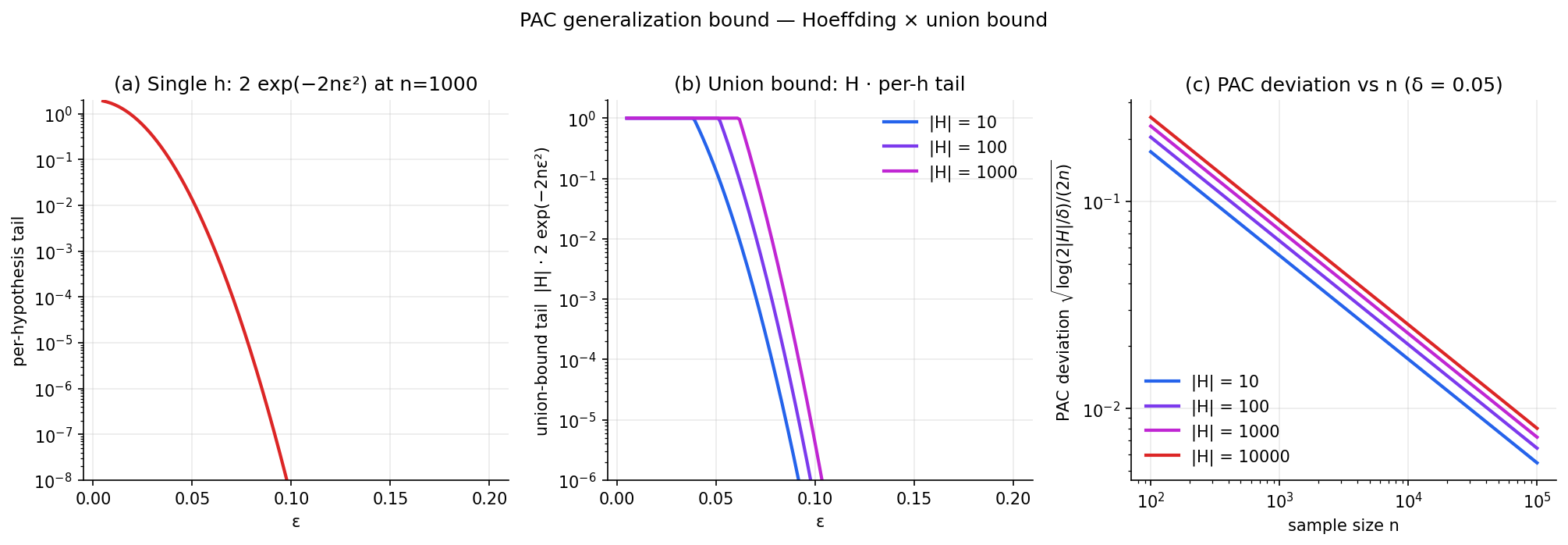
📝 Example 14 (The PAC generalization bound)
Let be a finite hypothesis class, and let be the training error of hypothesis on i.i.d. samples , with true risk . By Theorem 8 applied to :
With probability at least , simultaneously for every :
Let be the empirical risk minimizer (ERM), and let be the best-in-class hypothesis. Then with the same probability,
where . The first inequality uses the uniform bound on ; the second uses that minimizes ; the third uses the uniform bound on . So the ERM’s true risk is within of the best-in-class true risk — and shrinks like while growing only as .
This is the canonical PAC bound for finite hypothesis classes. Forward link: Generalization Bounds → formalML for VC dimension and Rademacher complexity, which replace with structural complexity measures for infinite classes.
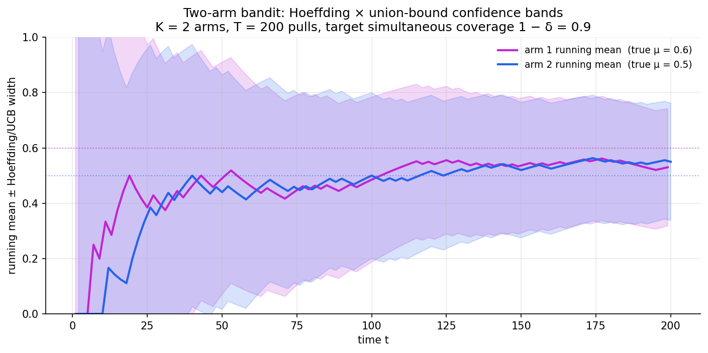
📝 Example 15 (UCB bandit confidence intervals)
In a -armed bandit, pulling arm at time produces a reward i.i.d. with unknown mean . After pulls of arm , the empirical mean is . By Hoeffding, for any :
The Upper-Confidence-Bound (UCB) algorithm pulls the arm with the largest . To guarantee simultaneous validity over all arms and time steps, set and apply Boole over the arm-time pairs: with probability , all confidence intervals are simultaneously valid throughout the horizon. The resulting confidence width is exactly the UCB exploration bonus.
Forward link: Multi-Armed Bandits → formalML, where the same construction is the core of the algorithm’s regret analysis.
10. Computational Notes
The inequalities of §§4–9 are useful precisely because they are computable. A few pragmatic notes on how the calculations work in practice — and where they fail numerically — follow.
-
Estimating P(A) by simulation. The empirical frequency is unbiased for and has standard error . By Hoeffding (Corollary 2), a distribution-free confidence interval is . NumPy idiom:
rng = np.random.default_rng(seed); samples = rng.uniform(0, 1, n); phat = np.mean(condition(samples)). -
Simulating Borel–Cantelli. Independent events with are drawn by
rng.uniform(0, 1, N) < p_n_array. The cumulative count stabilizes (BC-I) or diverges (BC-II) — this is the cleanest pedagogical demonstration of the dichotomy and is exactly what theBorelCantelliExplorerviz reproduces. -
Numerical pitfall: versus . When is small, both expressions are close — but the naive form in floating point can lose all significant digits to subtractive cancellation when and is moderate. Use
-numpy.expm1(-m * p)or the closely related1 - numpy.exp(-m * p)for the latter form, both of which are numerically stable. TheoneMinusOneMinusPToTheMhelper insrc/components/viz/shared/probability.tswraps this. -
scipy.statstail probabilities. For ascipy.stats.normrandom variable,1 - cdf(t)and the equivalent survival functionsf(t)return for the standard Gaussian. The notebook compares these exact tail values against Markov, Chebyshev, and Hoeffding bounds for several distributions — the Hoeffding bound is not applicable to Gaussians (unbounded support), which is why Markov on is replaced by sub-Gaussian arguments in formalML.
📝 Example 16 (Monte Carlo verification of the union bound)
A 10-line check on the flagship visualization’s claim. Place events as circular regions on the unit square with prescribed pairwise overlaps. Generate uniform samples on . The empirical is the fraction of samples falling in at least one circle; the union-bound estimate is the sum of the per-circle areas. Inclusion–exclusion gives the exact analytic value via the closed-form circle-intersection identity. The three quantities should satisfy
with the gap between the last two growing as the overlap grows. The companion notebook computes this for the three flagship presets and reports the ratio of the upper bound to the exact value — values near confirm tightness, values confirm looseness.
11. Connections to Statistics
The union bound is the single inequality that does more work in classical and modern statistics than any other.
-
Family-wise error rate control. Bonferroni’s procedure is the cleanest application of the union bound in all of statistics. Holm’s step-down procedure tightens Bonferroni by combining the union bound with a closed-testing principle, and remains a single-page proof. Both procedures control the family-wise error rate (FWER) at level regardless of dependence among the tests, at the cost of testing each hypothesis at level . Forward link: Multiple Testing and False Discovery → formalStatistics for FDR control (Benjamini–Hochberg), which sacrifices FWER for a softer error guarantee and a much higher discovery rate.
-
Confidence intervals from Hoeffding. For a sample mean of bounded random variables, the Hoeffding CI is distribution-free and exact (not asymptotic). This is the textbook “exact” CI used when normal approximations cannot be trusted, e.g., for small or when the underlying distribution is unknown. Forward link: Hypothesis Testing → formalStatistics.
-
Multi-arm A/B tests. Running simultaneous A/B tests with a shared overall error budget is a union-bound problem. The Bonferroni-corrected interval for the difference in means in each test gives a simultaneous confidence region for all differences. The same Hoeffding-plus-union-bound machinery from §9 underlies the modern always-valid sequential testing literature, where confidence intervals are valid at all stopping times rather than at a fixed sample size.
12. Connections to ML
The union bound is the bridge from probability to learning theory. Four threads, in increasing order of generality.
-
PAC learning and generalization bounds. The combination of Hoeffding (per-hypothesis concentration) and the union bound (over a finite hypothesis class) gives the canonical generalization bound for empirical risk minimization (Example 14). For infinite classes, the union bound is replaced by a covering / VC argument, but the structural idea — “convert per-event tails into uniform tails” — is preserved. Forward link: Generalization Bounds → formalML.
-
Multi-armed bandits. The UCB family of algorithms uses Hoeffding-plus-union-bound to construct simultaneous confidence intervals for arm means; the algorithm’s regret bound is a direct application of this construction (Example 15). Forward link: Multi-Armed Bandits → formalML.
-
Concentration inequalities, full hierarchy. Markov, Chebyshev, and Hoeffding are the foundational rungs of concentration. Sub-Gaussian and sub-exponential random variables (the next rungs) extend the MGF method introduced in §8 to unbounded variables with controlled tails. The Cramér–Chernoff method, Bernstein’s inequality, McDiarmid’s bounded-differences inequality, and Talagrand’s inequality all live downstream. Forward link: Concentration Inequalities → formalML.
-
Importance-sampling diagnostics. The effective sample size in importance sampling is monitored against the Hoeffding-style confidence width. When the importance weights are unbounded, Hoeffding breaks (its hypothesis fails) and one falls back to Chebyshev with the variance of the weights — a strictly looser bound. The connection between weight variance and tail control is one of the cleanest illustrations of why the Markov → Chebyshev → Hoeffding ladder matters. Forward link: Radon-Nikodym & Probability Densities (importance sampling section).
-
Sub-Gaussian noise in stochastic optimization. SGD’s convergence guarantees under bounded-noise assumptions reduce to applying Hoeffding to the noise sequence and then a union bound across iterations. The ” price of iterating” in SGD convergence theorems is exactly the tax from §9. Forward link: Concentration Inequalities → formalML.
📝 Example 17 (The PAC bound, numerically)
With , , , the deviation bound is
So with probability , the ERM hypothesis satisfies . The cost of “best of hypotheses” is a factor inside the square root — paid as a multiplier on the per-hypothesis deviation. Doubling the class to adds only to the deviation. The ” tax” is what makes finite-class PAC learning feasible at all.
Connections & Further Reading
Prerequisites — topics you need first
Sequences, Limits & Convergence
The limsup of sets, {A_n i.o.} = ∩_N ∪_{n≥N} A_n, is the event the Borel–Cantelli lemmas describe. Convergence of sequences of probabilities frames the asymptotic statements.
Series Convergence & Tests
First Borel–Cantelli requires Σ P(A_n) < ∞. Comparison and ratio tests classify scenarios in worked examples; the ladder of harmonic-like series shows where BC-I fails.
Improper Integrals & Special Functions
Continuous-RV statements of Markov, Chebyshev, and Hoeffding integrate against densities; the tail-integral identity E[X] = ∫₀^∞ P(X > t) dt motivates Markov geometrically.
Sigma-Algebras & Measures
(forward) The Kolmogorov axioms here are the finite/countable special case of the measure-theoretic foundations Topic 25 builds. Almost every claim proven here is generalized there.
The Lebesgue Integral
(forward) Markov's inequality for the Lebesgue integral is proved in Topic 26; the elementary version here is the special case.
Where this leads — next in formalCalculus
On to formalStatistics — where this calculus powers inference
Multiple Testing And False Discovery
The Bonferroni family-wise error rate bound and the Holm step-down procedure are both direct applications of the union bound proved in Section 4. The inclusion–exclusion structure of finite-sample p-value adjustments is the inequality in §5.
Hypothesis Testing
Markov and Chebyshev (Section 7) provide the elementary tail bounds that govern Type-I and Type-II error before any distributional assumption. Hoeffding (Section 8) is the bounded-RV upgrade testing arguments lean on.
On to formalML — where this calculus powers ML
Concentration Inequalities
Markov → Chebyshev → Hoeffding is the entry sequence to all of concentration. formalML's sub-Gaussian and sub-exponential bounds start from the MGF technique introduced in Section 8.
Generalization Bounds
The canonical PAC bound P(exists h in H : |R̂(h) − R(h)| > ε) ≤ |H| · 2 exp(−2nε²) is exactly the union bound applied across a hypothesis class with Hoeffding per hypothesis. This combination is built explicitly in Section 9.
Multi Armed Bandits
UCB confidence intervals are union bounds across arms and time. The 'union bound + tail concentration' pattern in §9 is the same machinery.
References
- book Grimmett & Stirzaker (2020). Probability and Random Processes Chapters 1–2. Standard reference for the axiomatic foundations at the level used here.
- book Rosenthal (2006). A First Look at Rigorous Probability Theory Chapters 1–3. The cleanest 'no-measure-theory-yet' treatment of axioms, conditional probability, and Borel–Cantelli.
- book Boucheron, Lugosi & Massart (2013). Concentration Inequalities: A Nonasymptotic Theory of Independence Chapters 2–3. The reference for Hoeffding's inequality, the MGF method, and the union-bound + concentration pattern.
- book Shalev-Shwartz & Ben-David (2014). Understanding Machine Learning: From Theory to Algorithms Chapter 4. The PAC generalization bound combining Hoeffding and the union bound; the canonical ML application.
- paper Hoeffding (1963). “Probability Inequalities for Sums of Bounded Random Variables” The original 1963 paper. The proof in Section 8 follows Hoeffding's argument.