Series Convergence & Tests
When do infinite sums make sense? The convergence tests that determine whether a series converges absolutely, conditionally, or not at all — and the learning rate conditions that make SGD work.
Abstract. An infinite series ∑ aₙ is defined as the limit of its partial sums Sₙ = a₁ + a₂ + ⋯ + aₙ — so series convergence is sequence convergence in disguise. The nth-term test provides a necessary condition (aₙ → 0), but the harmonic series ∑ 1/n shows it is not sufficient. The comparison test and limit comparison test relate unknown series to known benchmarks; the ratio test |aₙ₊₁/aₙ| → L and root test |aₙ|^(1/n) → L determine convergence when L < 1 and divergence when L > 1; the integral test connects ∑ f(n) to ∫ f(x)dx, bridging discrete sums and continuous integrals. For alternating series, the Leibniz test guarantees convergence when the terms decrease monotonically to zero. A series converges absolutely if ∑ |aₙ| converges, and absolute convergence implies convergence — but the converse fails: the alternating harmonic series ∑ (-1)ⁿ⁺¹/n converges conditionally but not absolutely. The Riemann rearrangement theorem reveals the fragility of conditional convergence: any conditionally convergent series can be rearranged to converge to any prescribed real number, or to diverge to ±∞. In machine learning, the Robbins-Monro conditions for SGD learning rates — ∑ αₜ = ∞ (the divergent series ensures the algorithm explores enough) and ∑ αₜ² < ∞ (the convergent series ensures the noise averages out) — are direct applications of series convergence theory. The p-series classification determines which polynomial-decay schedules αₜ = 1/tᵖ satisfy both conditions simultaneously: exactly those with p ∈ (1/2, 1]. The geometric series ∑ rⁿ = 1/(1-r) appears in discount factors for reinforcement learning, in the convergence analysis of momentum methods, and in the radius of convergence for power series that will be developed in the next topic.
1. Overview & Motivation
You’re training a neural network with stochastic gradient descent. The learning rate schedule controls how aggressively the model updates at step . The schedule must satisfy two competing demands: (the total step size must be infinite so the algorithm can reach any point in parameter space) and (the total squared step size must be finite so the noise averages out). These are the Robbins-Monro conditions, introduced as forward references in Sequences, Limits & Convergence. The question is: which values of satisfy both conditions simultaneously? The answer — — requires knowing when the -series converges and when it diverges. That is what this topic is about.
But learning rate schedules are just one instance of the fundamental question: when does an infinite sum converge to a finite value? The answer occupies a central position in analysis and in machine learning. Loss series, gradient accumulation bounds, discount factors in reinforcement learning, tail probabilities in concentration inequalities, and Fourier coefficients — all are governed by the convergence theory we develop here.
The key insight: an infinite series is not a new concept. It is a sequence — the sequence of partial sums . Every tool from Sequences, Limits & Convergence applies directly. We are not learning new machinery. We are applying existing machinery to a new and important class of sequences.
2. From Sequences to Series
An infinite series is a sequence in disguise. Every question about the convergence of is really a question about the convergence of the sequence where . This is not a metaphor — it is the definition.
📐 Definition 1 (Infinite Series)
Given a sequence in , the infinite series is the sequence of partial sums defined by
The terms are the terms of the series and is the th partial sum.
📐 Definition 2 (Convergence of a Series)
The series converges if the sequence of partial sums converges — that is, if exists as a finite real number. We write and call the sum of the series. If does not converge, the series diverges.
💡 Remark 1 (The reduction principle)
Definitions 1 and 2 convert every series problem into a sequence problem. The Monotone Convergence Theorem, the Cauchy criterion, and the Algebra of Limits — all from Sequences, Limits & Convergence — now apply to partial sums. In particular:
(a) If all , then is increasing, so converges iff is bounded (Monotone Convergence).
(b) converges iff for every there exists such that for all (Cauchy criterion for series).
The first convergence test is an immediate consequence:
🔷 Theorem 1 (The Divergence Test (nth-Term Test))
If converges, then .
Equivalently (contrapositive): if , then diverges.
Proof.
If the series converges with sum , then and . Since , the Algebra of Limits gives .
💡 Remark 2 (The divergence test is necessary but not sufficient)
The harmonic series has , but it diverges (we prove this in the next section). Having is necessary for convergence, but far from sufficient. The convergence tests in the following sections provide stronger criteria. The divergence of is also what makes the second Borel–Cantelli lemma produce a probability-1 “infinitely often” event in Probability & The Union Bound; the convergence of produces the probability-0 version.
The interactive explorer below makes the “series = sequence of partial sums” reduction tangible. Select a series preset and watch the partial sums converge (or not) as increases. For convergent series, drag the slider to see the - definition in action — the same definition from Sequences, Limits & Convergence, now applied to the partial-sum sequence.
3. Fundamental Series — Geometric & -Series
Every convergence test works by comparing an unknown series to one of two benchmark families. These benchmarks are the reference points of series theory.
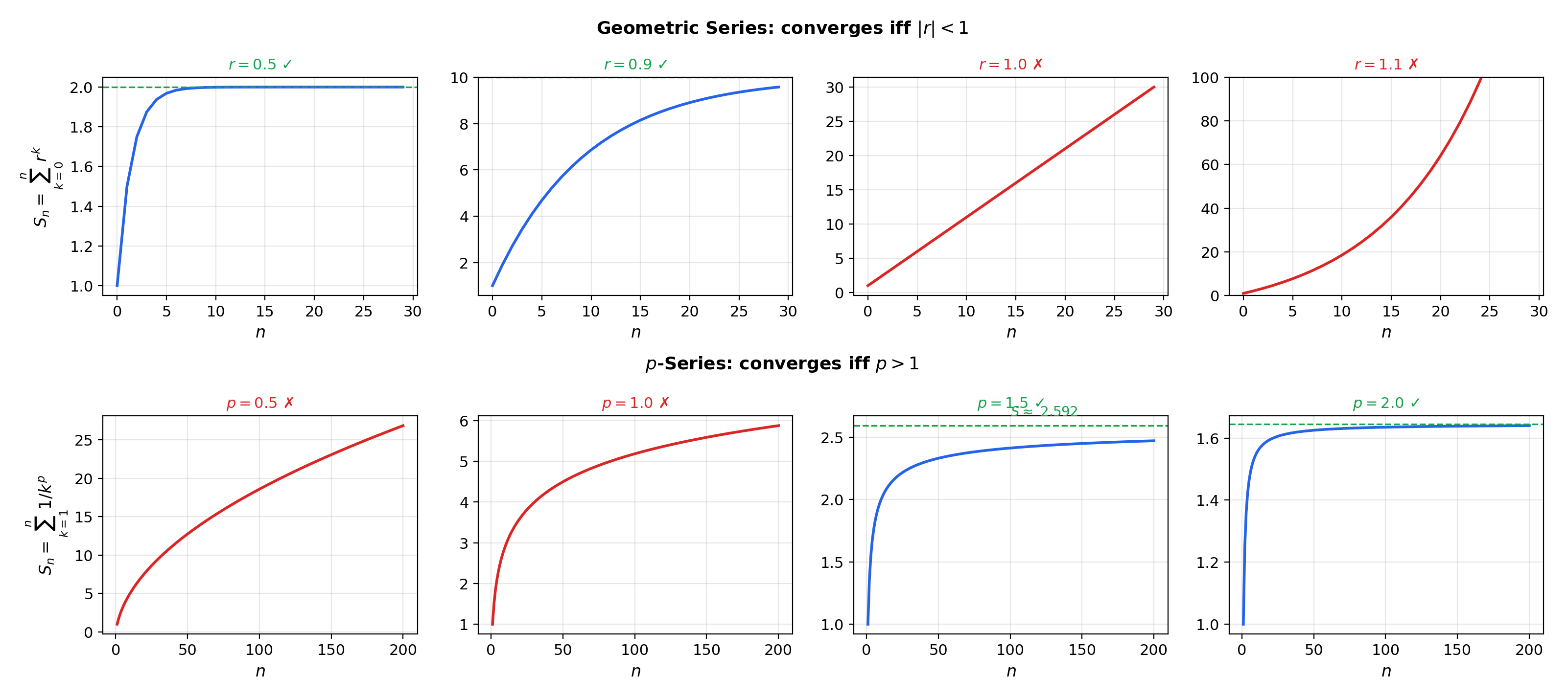
🔷 Theorem 2 (The Geometric Series)
For :
Proof.
The partial sum has the closed form (verified by multiplying both sides by and telescoping). If , then (from Sequences, Limits & Convergence, the sequence for ), so . If , then , so does not converge.
💡 Remark 3 (Why the geometric series matters)
The geometric series is the most important series in mathematics and in ML. In reinforcement learning, the discounted return is a geometric series weighted by rewards — convergence requires , which is why discount factors satisfy . In momentum-based optimization (e.g., Adam), the bias correction factor is the geometric series sum. In the ratio test (Theorem 6), convergence is established by showing the terms eventually decay faster than a geometric series.
📝 Example 1 (Geometric series computations)
(a) .
(b) .
(c) .
📐 Definition 3 (The p-Series)
For , the -series is .
🔷 Theorem 3 (p-Series Convergence)
converges if and only if .
Proof.
We use the Cauchy condensation test. Consider the “condensed” series . This is a geometric series with ratio , which converges iff , i.e., , i.e., .
The Cauchy condensation theorem states: for a positive decreasing sequence , converges iff converges. The key idea is that the block of terms contains terms, each between and (since the sequence is decreasing). So the block sum is bounded between and , and the condensed series captures the growth rate exactly.
📝 Example 2 (The harmonic series diverges)
Setting : .
Alternative proof (Oresme’s grouping):
Each group of terms sums to at least , so the partial sums grow without bound. This is perhaps the most important divergence result in analysis — it says that even though , the terms don’t shrink fast enough to produce a finite sum.
📝 Example 3 (p-series classification)
- (Basel problem, converges — ).
- converges ().
- diverges ().
4. Comparison Tests
The comparison tests let us determine convergence by bounding an unknown series against a known benchmark.
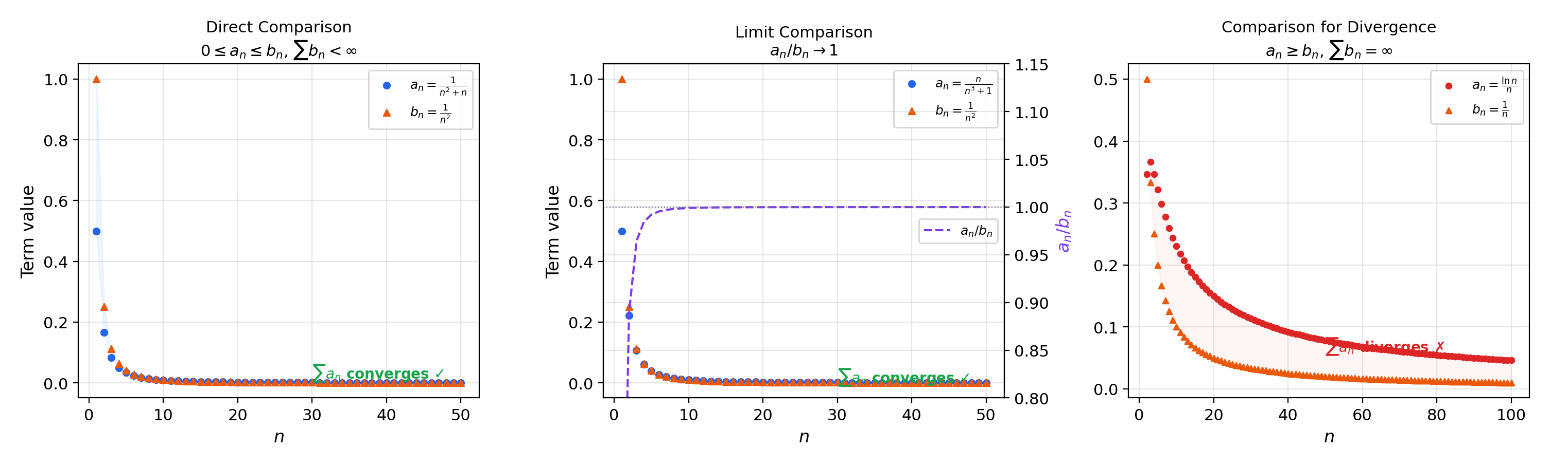
🔷 Theorem 4 (The Comparison Test (Direct))
Let for all . Then:
- If converges, then converges.
- If diverges, then diverges.
Proof.
(1) The partial sums are increasing (since ) and bounded above by . By the Monotone Convergence Theorem (Sequences, Limits & Convergence, Theorem 1), converges.
(2) Contrapositive of (1).
📝 Example 4 (Using the comparison test)
(a) converges: and converges.
(b) diverges: for and diverges.
🔷 Theorem 5 (The Limit Comparison Test)
Let and for all . If where , then and either both converge or both diverge.
Proof.
Since , for there exists such that . Thus for all . If converges, the direct comparison gives , so converges. If diverges, then .
📝 Example 5 (Limit comparison)
converges: compare with , since , and converges.
💡 Remark 4 (The comparison hierarchy)
The direct comparison test requires an explicit inequality or , which can be algebraically demanding. The limit comparison test requires only that asymptotically, which is usually easier to verify. In practice, the limit comparison test with -series benchmarks handles most polynomial-type series.
5. Ratio & Root Tests
The comparison tests require an external benchmark series. The ratio and root tests are self-contained: they use the series’s own terms to determine convergence by detecting whether the terms eventually decay faster than a geometric series.
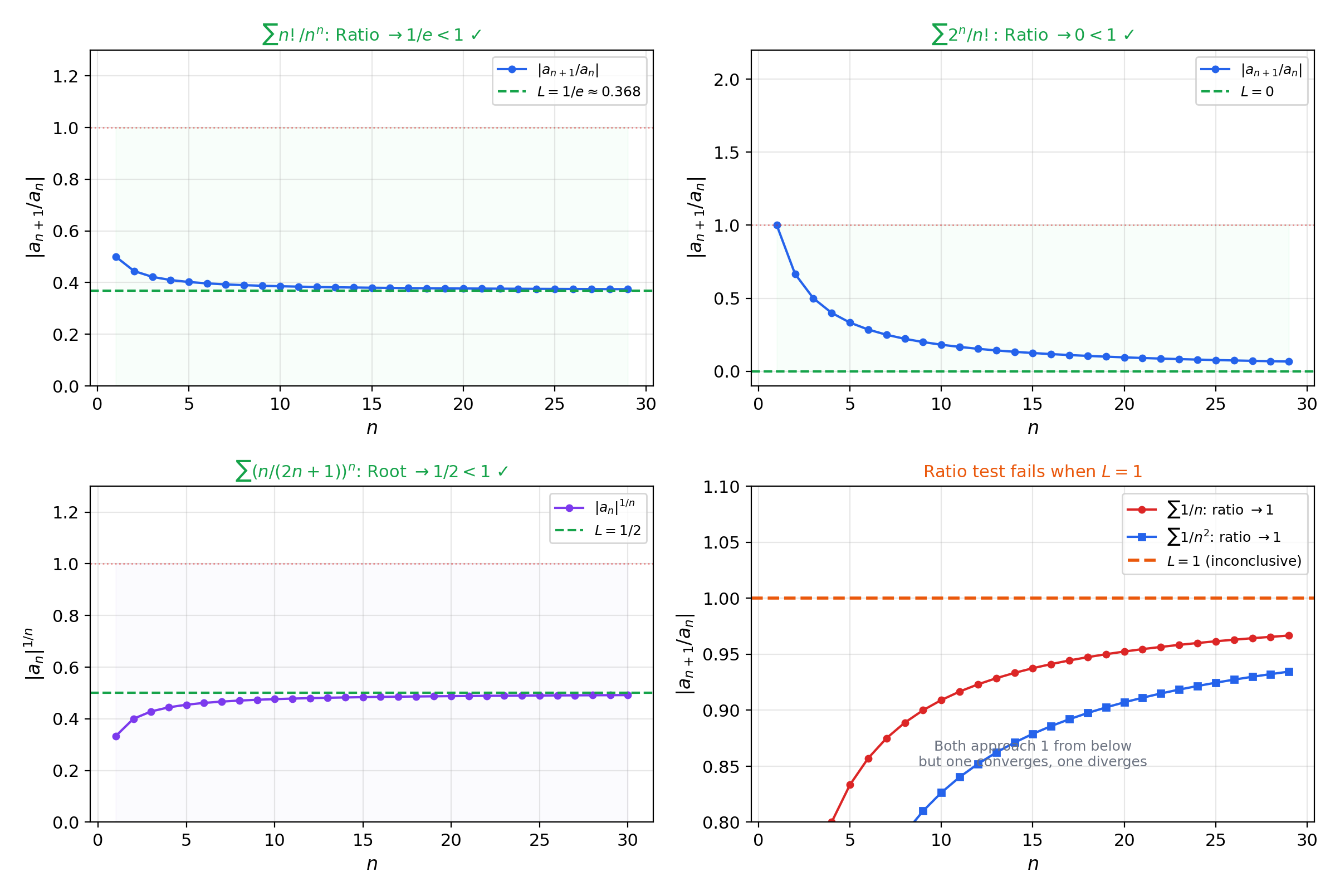
🔷 Theorem 6 (The Ratio Test (d'Alembert))
Let be a sequence with for all . Define (if the limit exists, or use ).
- If , the series converges absolutely.
- If (or ), the series diverges.
- If , the test is inconclusive.
Proof.
(1) If , choose with . By definition of the limit, there exists such that for all . Then for (by induction). Since is a convergent geometric series (), the comparison test gives .
(2) If , eventually , so is eventually increasing and . The series diverges by the divergence test.
📝 Example 6 (Ratio test applications)
(a) : . Converges.
(b) : . Converges.
(c) : . Inconclusive (we know it diverges by other means).
🔷 Theorem 7 (The Root Test (Cauchy))
Let .
- If , the series converges absolutely.
- If , the series diverges.
- If , the test is inconclusive.
Proof.
(1) If , choose with . By definition of , there exists such that for all (this is where is needed rather than — there may be finitely many exceptions). Then for all , and (convergent geometric series).
(2) If , then for infinitely many , so for infinitely many , hence .
📝 Example 7 (Root test applications)
(a) : . Converges.
(b) : . Converges.
💡 Remark 5 (Ratio vs. root — root is strictly stronger)
The root test is strictly stronger than the ratio test: whenever the ratio test gives a verdict, the root test gives the same verdict, but there exist series where the root test succeeds and the ratio test is inconclusive. This is because . In practice, the ratio test is more convenient for factorials and exponentials, while the root test is better for th powers.
The convergence test dashboard below applies multiple tests to the same series simultaneously, showing which tests are conclusive and which are not. This makes the relative power of the tests visible — the root test never fails when the ratio test succeeds, but sometimes succeeds when the ratio test gives up.
6. The Integral Test
The integral test connects series convergence to improper integral convergence — linking the discrete world of to the continuous world of from Improper Integrals & Special Functions.
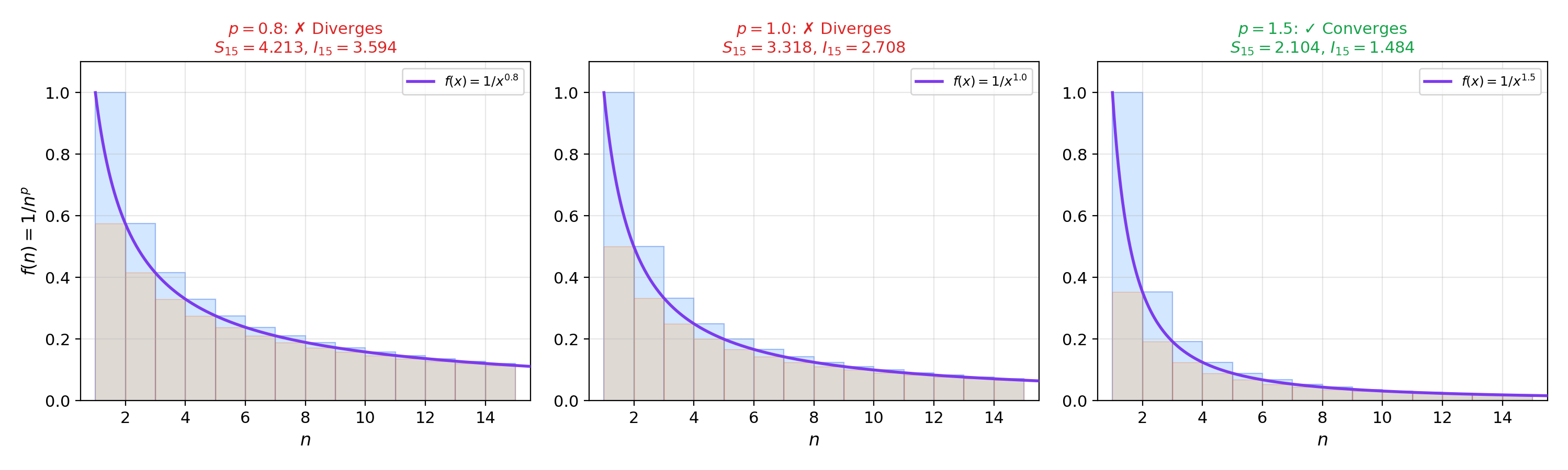
The geometric idea is clean. If is positive, continuous, and decreasing on , the rectangles of height and width 1 overestimate or underestimate the area under . Specifically:
So the partial sums and the integrals are bounded by each other — they converge or diverge together.
🔷 Theorem 8 (The Integral Test)
Let be positive, continuous, and decreasing. Then converges if and only if converges.
Proof.
Since is decreasing, for all : . Summing from to :
If converges, the right inequality gives , so is bounded and increasing, hence convergent by the Monotone Convergence Theorem. If , the left inequality gives , so the partial sums diverge.
📝 Example 8 (The integral test recovers p-series)
For : , which converges iff , i.e., . This recovers Theorem 3 via the integral test.
📝 Example 9 (Series not amenable to other tests)
for : the ratio and root tests both give (inconclusive). The integral test with : substituting ,
Converges. This is a series that only the integral test can handle among our toolkit.
💡 Remark 6 (Integral test remainder bounds)
The integral test also provides error bounds: if is the remainder after terms, then
This tells you how many terms you need for a given accuracy — exactly the kind of bound used in numerical analysis and in bounding truncation error in series approximations for ML (e.g., truncating a Taylor expansion or a Fourier series).
7. Alternating Series & the Leibniz Test
In all the tests so far, we have mostly dealt with series of positive terms. Alternating series — where the signs alternate — introduce a fundamentally new phenomenon: cancellation between positive and negative terms can produce convergence even when the series of absolute values diverges.
📐 Definition 4 (Alternating Series)
A series where for all is an alternating series.
🔷 Theorem 9 (The Alternating Series Test (Leibniz Test))
If is decreasing () and , then the alternating series converges.
Proof.
Consider the even partial sums:
Each parenthesized pair is (since is decreasing), so is increasing. Also,
so is bounded above by .
By the Monotone Convergence Theorem, for some . Now . Since both the even and odd subsequences converge to , the full sequence .
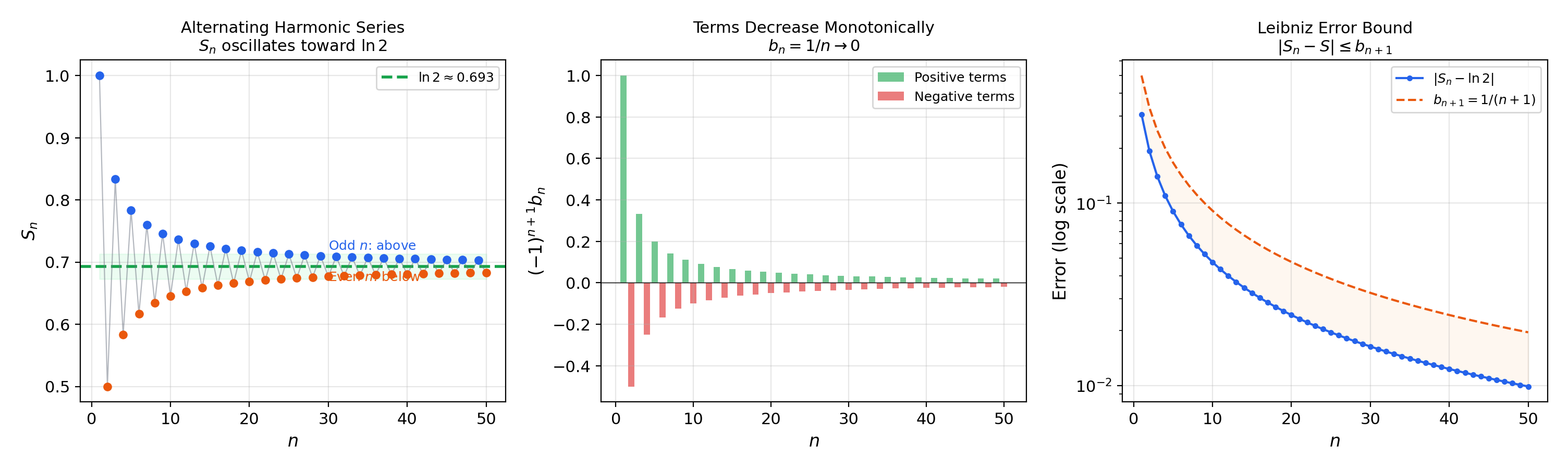
📝 Example 10 (The alternating harmonic series)
. The terms are decreasing and tend to , so the Leibniz test applies. The sum is (provable via the Taylor series of at , which we establish in Power Series & Taylor Series).
Note: diverges, so this series converges conditionally but not absolutely. We formalize this distinction in the next section.
💡 Remark 7 (Alternating series remainder)
If the alternating series converges to , the error after terms satisfies — the error is bounded by the first omitted term. This is a remarkably tight bound, much better than what most convergence tests provide.
8. Absolute vs. Conditional Convergence
Absolute convergence is the “safe” mode of convergence — it is robust under rearrangement and implies all forms of convergence. Conditional convergence is fragile: rearranging the terms can change the sum or destroy convergence entirely.
📐 Definition 5 (Absolute Convergence)
A series converges absolutely if converges.
📐 Definition 6 (Conditional Convergence)
A series converges conditionally if it converges but does not converge absolutely — that is, converges but .
🔷 Theorem 10 (Absolute Convergence Implies Convergence)
If converges, then converges, and .
Proof.
We use the Cauchy criterion. Since converges, for any there exists such that for all . By the triangle inequality:
This is the Cauchy criterion for , so converges.
The inequality follows by taking limits of where .
Note: This proof uses the completeness of — the Cauchy criterion requires completeness. In an incomplete space (like ), absolute convergence need not imply convergence. See Completeness & Compactness for why completeness matters.
📝 Example 11 (Classification)
(a) converges absolutely ().
(b) converges conditionally (, but the Leibniz test gives convergence).
(c) diverges (not even conditional convergence — the th-term test kills it).
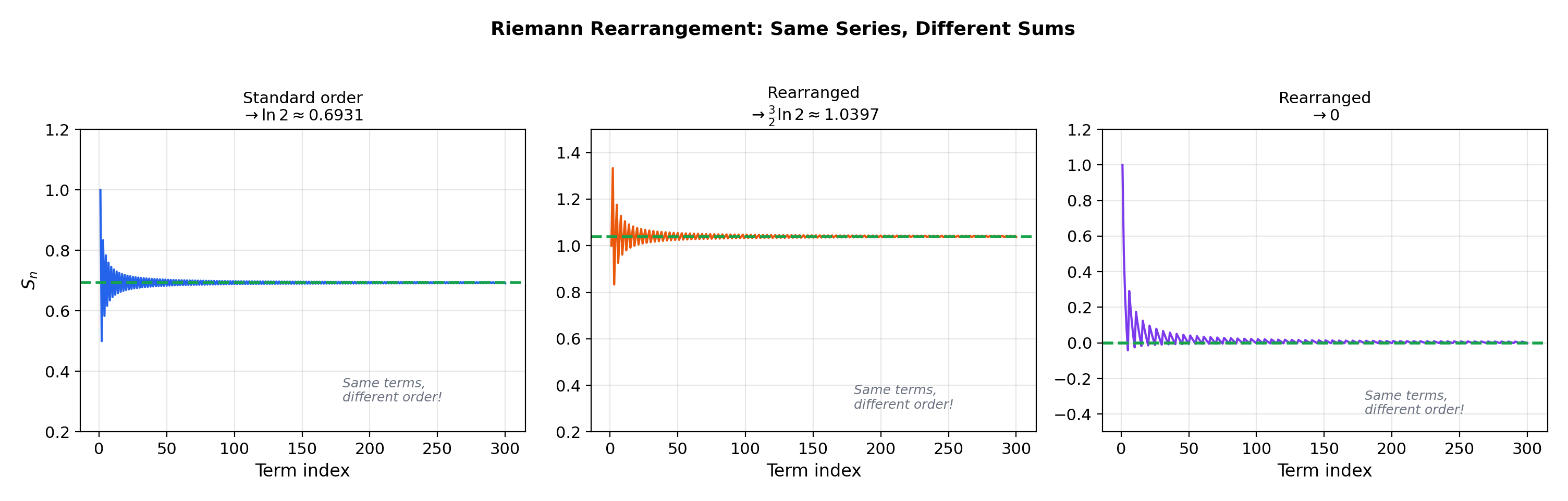
🔷 Theorem 11 (The Riemann Rearrangement Theorem)
Let be a conditionally convergent series. Then for any , there exists a rearrangement (where is a bijection) that converges to .
Proof.
Let be the positive terms (in their original order) and the negative terms. Since is conditionally convergent, both and — if either were finite, the series would converge absolutely.
To reach a target : add positive terms until the partial sum first exceeds ; then add negative terms until it drops below ; then add more positive terms until it exceeds again; continue alternating.
The key insight: because and (since by the divergence test applied to the original convergent series), each overshoot/undershoot gets smaller. The partial sums oscillate around with decreasing amplitude, converging to by the squeeze theorem.
💡 Remark 8 (Rearrangement and absolute convergence)
If converges absolutely, then every rearrangement converges to the same sum. This is why absolute convergence is the “safe” mode: it is invariant under permutation. Conditional convergence is inherently order-dependent.
In computational settings, finite-precision arithmetic implicitly rearranges series (due to rounding and the order of evaluation), so absolute convergence guarantees reproducibility, whereas conditional convergence does not.
📝 Example 12 (A rearrangement of the alternating harmonic series)
The standard ordering gives .
The rearrangement (two positive terms, then one negative term) converges to .
The explorer below shows absolute vs. conditional convergence side by side, and lets you construct Riemann rearrangements that converge to different target values — demonstrating the theorem in real time.
9. A Test Selection Guide
With seven convergence tests in hand, we need a decision framework.
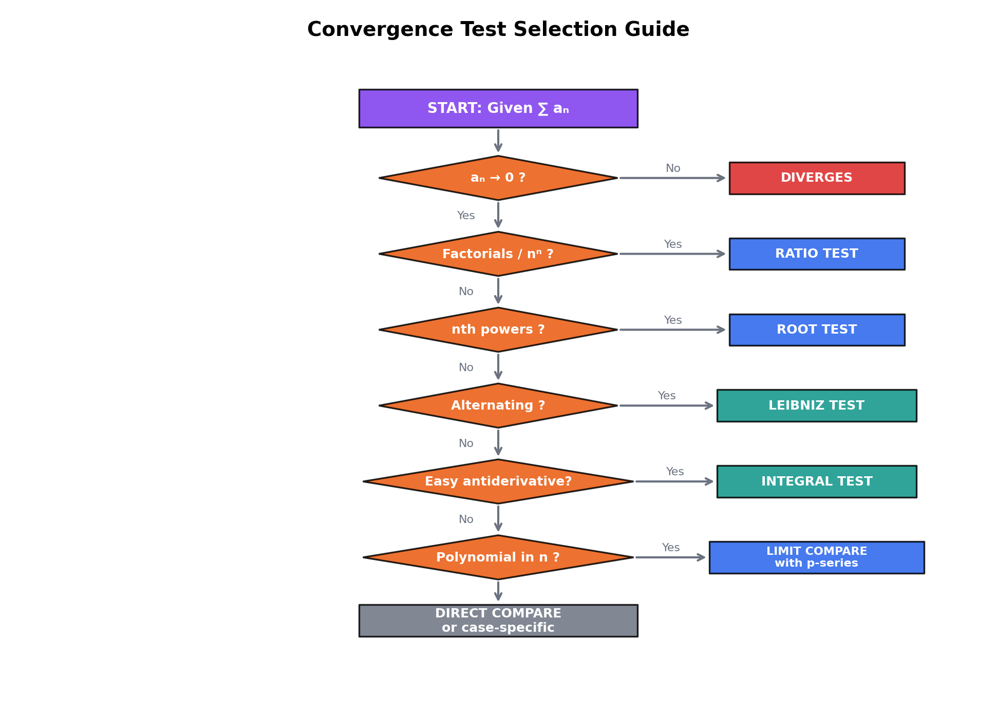
💡 Remark 9 (Test selection strategy)
- Always check the divergence test first. If , the series diverges — done.
- Recognize geometric series () and -series () immediately. These are the benchmarks.
- Factorials or th powers of constants: ratio test.
- th powers of -dependent expressions: root test.
- Series resembling asymptotically: limit comparison with the -series.
- where has an elementary antiderivative: integral test.
- Alternating series: Leibniz test.
- If you need absolute convergence: apply tests 3–6 to .
10. Computational Notes
In practice, we compute partial sums with NumPy and verify convergence tests numerically. The following patterns appear constantly in ML and scientific computing.
Computing partial sums. Given a term function a(n), the partial sums are np.cumsum([a(n) for n in range(1, N+1)]). For the geometric series with and , this gives a value within of the exact sum .
Numerical ratio test. Compute |a(n+1)/a(n)| for up to and plot the sequence. If it stabilizes below , the series converges; above , it diverges; near , look elsewhere.
Numerical root test. Compute |a(n)|^(1/n) and plot. This is more numerically stable for series with th powers, since taking the th root normalizes the growth rate.
Integral test with scipy.integrate.quad. For , quad(f, 2, np.inf) returns , confirming convergence.
Riemann rearrangement. Alternating between positive and negative terms of the harmonic series, targeting a value : the algorithm described in Theorem 11’s proof is directly implementable and converges to any target within after using terms.
11. Connections to Statistics
Series convergence is the analytical engine for almost-sure convergence proofs, generating-function methods, and large-deviation asymptotics.
Borel–Cantelli and almost-sure convergence
The Borel–Cantelli lemma — if then — is a series-convergence statement translated into probability. Almost-sure convergence proofs in statistics routinely reduce to showing an appropriate series converges. See formalStatistics Modes of Convergence.
Generating functions
The probability generating function is a power series whose coefficients are the PMF values. Moment generating functions and cumulant generating functions are Laurent/Taylor series whose coefficients encode the distribution; whether they exist on a neighborhood of is exactly a series-convergence question. See formalStatistics Discrete Distributions.
Edgeworth expansions and rate functions
Edgeworth expansions give higher-order corrections to the CLT — asymptotic series whose convergence properties determine when higher-order approximations (including the bootstrap) are accurate. In large-deviation theory, is a power series whose Legendre transform is the rate function; series convergence determines its domain. See formalStatistics Central Limit Theorem and formalStatistics Large Deviations.
12. Connections to ML
Series convergence appears in ML through four distinct paths.
11.1 Learning Rate Schedules & the Robbins-Monro Conditions
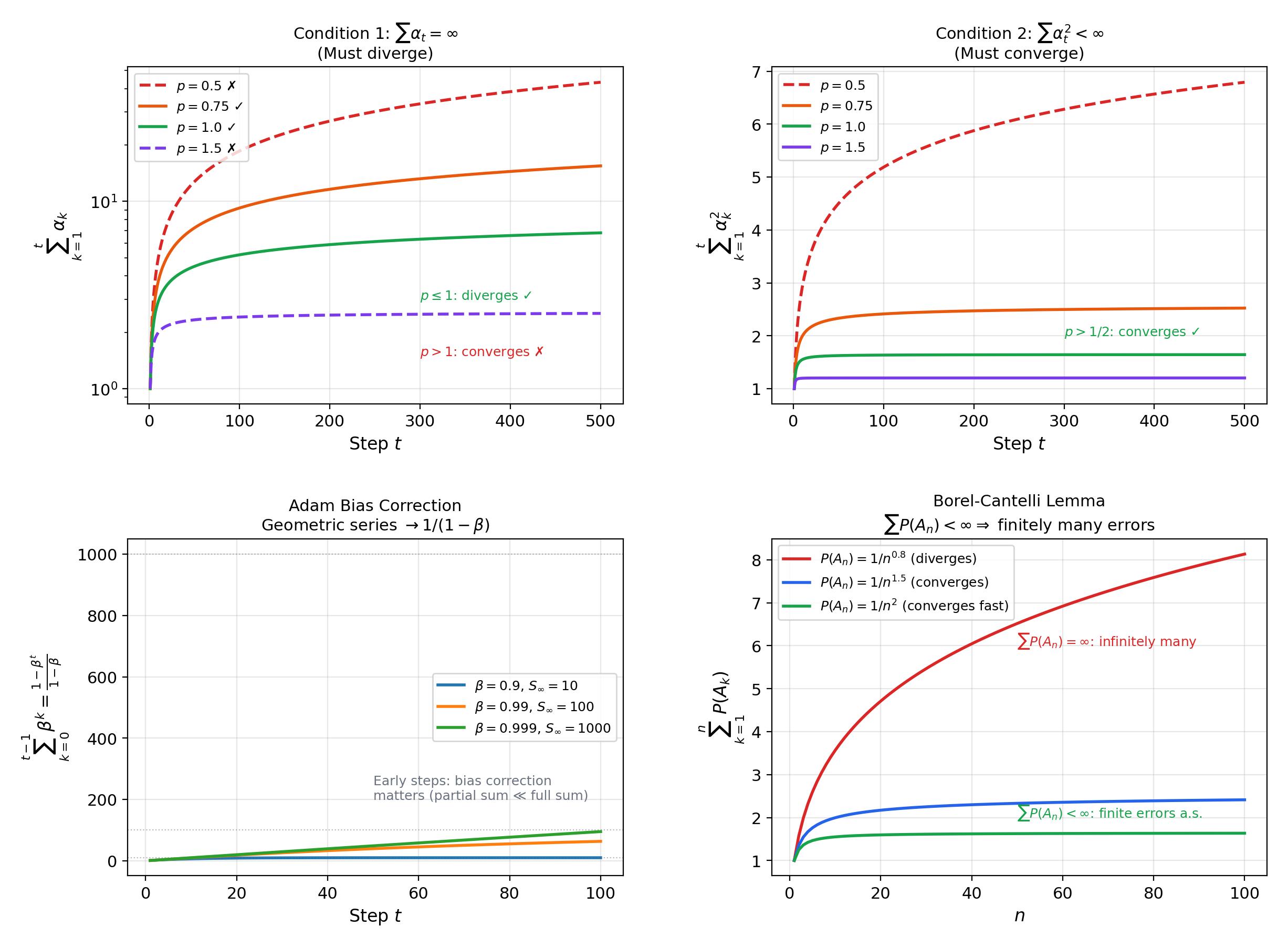
The Robbins-Monro conditions for SGD: and . The first condition ensures the algorithm can reach any point (the total step size is unbounded). The second ensures that the noise variance remains finite (the iterates don’t oscillate forever).
For polynomial schedules : converges iff (Theorem 3), and converges iff , i.e., . Both conditions are satisfied iff . The canonical choice () satisfies both conditions exactly at the boundary.
For exponential schedules with : (geometric series), so condition 1 fails — the algorithm stops exploring too soon. This is why exponential decay schedules require warmup or restarts in practice.
-> Gradient Descent -> formalML
11.2 Gradient Accumulation & Momentum
In momentum-based optimizers (SGD with momentum, Adam), the update at step is a weighted sum of all past gradients: . The total weight is the partial sum of a geometric series: . As , this approaches . Adam’s bias correction divides by precisely to account for the finite partial sum being less than the infinite series sum.
11.3 Discount Factors in Reinforcement Learning
The discounted return is a geometric series in the discount factor . The series converges because , and the total weight is . If rewards are bounded by , then .
11.4 The Borel-Cantelli Lemma in Online Learning
The first Borel-Cantelli lemma: if , then — only finitely many of the events occur almost surely. In online learning, if is the event “the algorithm makes an error at step ,” and the error probabilities decrease fast enough that their series converges, then the total number of errors is finite almost surely. The convergence test used to verify is typically comparison with a -series.
-> Measure-Theoretic Probability -> formalML
-> PAC Learning -> formalML
Connections & Further Reading
Prerequisites — topics you need first
Uniform Convergence
The Weierstrass M-test (Topic 4, Theorem 4) is a series convergence test for function series: if |gₖ(x)| ≤ Mₖ and ∑Mₖ converges, then ∑gₖ converges uniformly. This topic provides the numerical convergence tests (comparison, ratio, root) used to verify ∑Mₖ < ∞.
Sequences, Limits & Convergence
Series convergence is sequence convergence. The partial sums Sₙ = ∑ₖ₌₁ⁿ aₖ form a sequence, and the series converges iff this sequence converges. Every convergence test reduces to applying the sequence theorems from Topic 1 — Monotone Convergence, Cauchy criterion, comparison — to the partial-sum sequence.
Improper Integrals & Special Functions
The integral test connects ∑f(n) to ∫₁^∞ f(x)dx: both converge, or both diverge when f is positive, continuous, and decreasing. This bridges the discrete (series) and continuous (improper integral) worlds, and the p-series/p-integral parallel is the central example.
Completeness & Compactness
Absolute convergence implies convergence because ℝ is complete: the partial sums of |aₙ| form a bounded monotone sequence (hence Cauchy), and the partial sums of aₙ are then Cauchy because |Sₘ - Sₙ| ≤ ∑|aₖ|. Without completeness, this argument fails.
The Riemann Integral & FTC
Riemann sums ∑f(xₖ*)Δxₖ are finite series that converge to the integral as the partition refines. The integral test reverses this relationship: it uses the integral to determine whether the related series converges.
Where this leads — next in formalCalculus
Power Series & Taylor Series
The ratio and root tests determine the radius of convergence; absolute convergence on the interior of the interval is established using the tests developed here.
Fourier Series & Orthogonal Expansions
Convergence of Fourier coefficients requires summability methods that generalize the convergence tests here — Bessel's inequality is a series-convergence statement about coefficient sequences.
Approximation Theory
Stone-Weierstrass and uniform convergence of approximating series. The convergence rates of Bernstein and Chebyshev expansions invoke the comparison and ratio tools developed here.
Sigma-Algebras & Measures
Countable additivity of measures is defined via convergent series; the Borel-Cantelli lemma is a series convergence test recast as a probabilistic statement about tail events.
Probability & The Union Bound
On to formalStatistics — where this calculus powers inference
Modes Of Convergence
Borel–Cantelli — if Σ P(A_n) < ∞ then P(A_n i.o.) = 0 — is a series-convergence statement translated into probability. Almost-sure convergence proofs routinely reduce to showing an appropriate series converges.
Discrete Distributions
The probability generating function G_X(s) = E[s^X] = Σ p_k s^k is a power series whose coefficients are the PMF values. Moment generating functions and cumulant generating functions are Laurent/Taylor series whose coefficients encode the distribution.
Central Limit Theorem
Edgeworth expansions give higher-order corrections to the CLT: F_n(x) = Φ(x) + n^(-1/2) p_1(x) φ(x) + n^(-1) p_2(x) φ(x) + ... — an asymptotic series whose convergence properties determine when higher-order approximations (including the bootstrap) are accurate.
Large Deviations
The cumulant generating function Λ(t) = log E[e^(tX)] is a power series (when convergent) whose coefficients are the cumulants. Cramér's theorem uses Λ and its Legendre transform; series convergence determines the domain of the rate function.
Law Of Large Numbers
The Borel–Cantelli lemma — used in both Etemadi's truncation step and the Glivenko–Cantelli theorem — requires $\sum P(A_n) < \infty$, a series-convergence condition. The variance series $\sum \mathrm{Var}(X_k)$ controls partial-sum behavior and feeds Kolmogorov's three-series theorem; both are direct applications of series-convergence theory.
On to formalML — where this calculus powers ML
Gradient Descent
The Robbins-Monro conditions for SGD learning rates — ∑αₜ = ∞ and ∑αₜ² < ∞ — are series convergence conditions. The p-series classification ∑1/tᵖ determines which polynomial-decay schedules satisfy both constraints: exactly p ∈ (1/2, 1].
PAC Learning
The union bound converts uniform convergence over a hypothesis class into a series ∑P(bad event for h). Finite VC dimension ensures this series is controlled, yielding generalization bounds.
Concentration Inequalities
Chernoff bounds produce geometric series in tail probabilities. The ratio test applied to moment-generating function expansions determines the strength of exponential concentration.
Measure Theoretic Probability
The Borel-Cantelli lemma — if ∑P(Aₙ) < ∞ then P(limsup Aₙ) = 0 — is a direct application of series convergence to probability theory. Countable additivity of measures is defined via convergent series of set measures.
References
- book Rudin (1976). Principles of Mathematical Analysis Chapter 3 — the definitive treatment of numerical series, convergence tests, and absolute vs. conditional convergence
- book Abbott (2015). Understanding Analysis Chapter 2 — an accessible treatment emphasizing the sequence-to-series reduction and the role of completeness
- book Folland (1999). Real Analysis: Modern Techniques and Their Applications Section 0.5 — series convergence in the context of measure theory prerequisites
- book Spivak (2008). Calculus Chapter 22 — series of real numbers with historically motivated exposition and complete proofs of all standard tests
- book Bartle & Sherbert (2011). Introduction to Real Analysis Chapter 3.7 and Chapter 9 — series convergence tests with careful comparison to improper integrals
- paper Robbins & Monro (1951). “A Stochastic Approximation Method” The original conditions ∑αₙ = ∞, ∑αₙ² < ∞ for stochastic approximation convergence — the foundational ML application of series convergence
- paper Kingma & Ba (2015). “Adam: A Method for Stochastic Optimization” Bias correction in Adam uses geometric series ∑βᵗ = 1/(1-β). Learning rate scheduling analysis requires the series tools from this topic.