Uniform Convergence
When do limits of functions inherit the properties of the functions themselves? The sup-norm, the ε/3 trick, the Weierstrass M-test, Arzelà-Ascoli, and the uniform convergence framework that makes PAC learning possible
Abstract. A sequence of functions (f_n) converges pointwise to f on D if for each x in D, f_n(x) converges to f(x) as n tends to infinity. But pointwise convergence is deceptively weak: the limit of continuous functions can be discontinuous (f_n(x) = x^n on [0,1] converges pointwise to a step function), integration and limits cannot be interchanged (a moving bump with constant integral can converge pointwise to zero), and derivatives of the limit may bear no relation to the limits of the derivatives. Uniform convergence fixes these pathologies by requiring that the convergence rate be independent of x: (f_n) converges uniformly to f if for every epsilon > 0, there exists N such that |f_n(x) - f(x)| < epsilon for ALL x in D simultaneously — equivalently, the sup-norm ||f_n - f||_infinity tends to zero. The Uniform Limit Theorem guarantees that the uniform limit of continuous functions is continuous (the epsilon/3 argument), and uniform convergence permits interchange of limits with Riemann integration. The Weierstrass M-test provides a practical criterion: if |g_k(x)| <= M_k for all x and the sum of M_k converges, then the series of g_k converges uniformly. The Arzela-Ascoli theorem characterizes compact subsets of C([a,b]) via equicontinuity and pointwise boundedness — it is the compactness theorem for function spaces, extending the Heine-Borel theorem from R^n to infinite-dimensional spaces. In machine learning, uniform convergence is the mathematical backbone of generalization theory. PAC learning guarantees that the empirical risk R_hat(h) converges uniformly to the true risk R(h) over a hypothesis class H, and the VC dimension controls the rate of this uniform convergence. The Glivenko-Cantelli theorem — the empirical CDF converges uniformly to the true CDF — is the foundational uniform convergence result in statistics.
Overview & Motivation
You’re training a neural network with increasing width: neurons per hidden layer. Each is a continuous function — compositions of affine maps and continuous activations like ReLU or sigmoid. As , does converge to some function ? And if so, is still continuous? Can you integrate by integrating the ? Can you differentiate by differentiating the ?
The answers depend on how converges — and the wrong notion of convergence gives the wrong answers to all three questions.
In Sequences, Limits & Convergence, we studied convergence of sequences of numbers: given a sequence in , does ? In Epsilon-Delta & Continuity, we studied continuity of individual functions: is continuous at ? In Completeness & Compactness, we studied structural properties that guarantee limits exist and optima are attained. Now we combine all three: when does a sequence of functions converge, and when does the limit inherit the properties of the functions themselves?
The answer will require a new notion of convergence — uniform convergence — that is strictly stronger than the naive “pointwise” approach. The distinction between these two notions is not a technicality. It is the mathematical backbone of generalization theory in machine learning.
Pointwise Convergence of Function Sequences
The simplest way to define convergence of a function sequence is to check convergence at each point separately.
📐 Definition 1 (Pointwise Convergence of Function Sequences)
A sequence of functions where converges pointwise to if for every ,
Equivalently, for every and every , there exists (which may depend on both and ) such that
The crucial phrase is “which may depend on both and .” We write to emphasize this dependence. At each fixed , we’re just asking for ordinary sequence convergence — the - definition from Sequences, Limits & Convergence. But the required might be very different at different points .
The canonical example makes this concrete:
📝 Example 1
Consider on . The pointwise limit is
Proof. For , we have , so as (geometric sequence with ratio ). For , we have for all .
Notice what happened: each is continuous on , but the pointwise limit has a jump discontinuity at . The limit of continuous functions is not continuous.
A second example where things go right: on also converges pointwise to (the same limit for ; at , ). And this time the limit is continuous. What’s different?
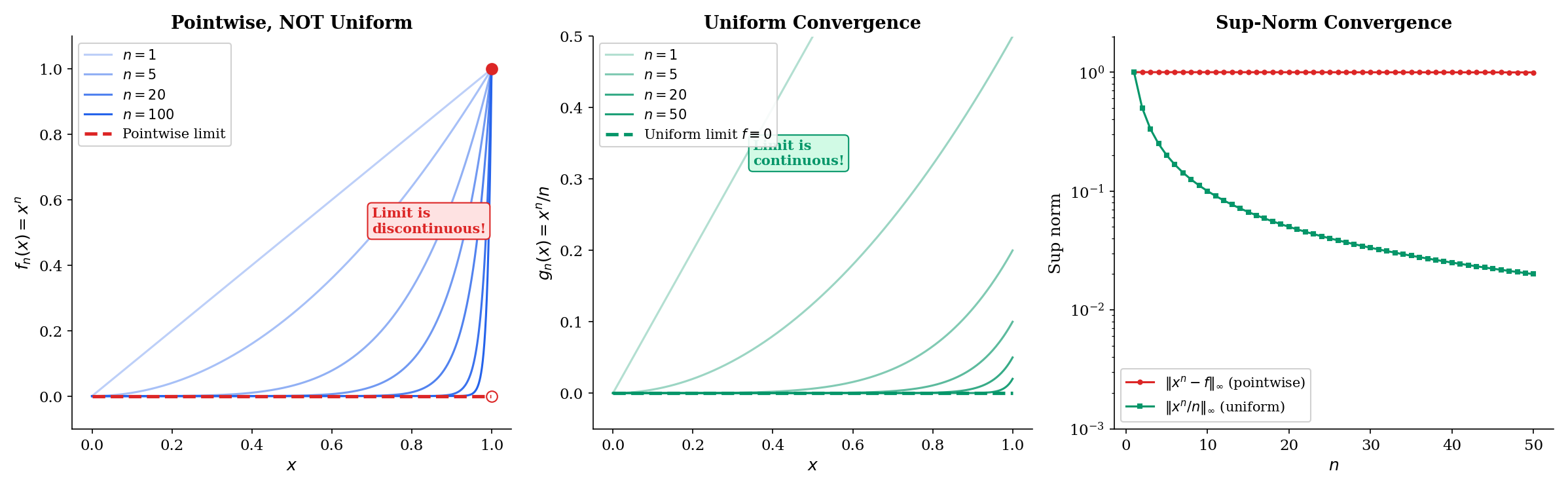
The difference is the convergence rate. For , points near require enormous to get close to the limit — as . For , the sup-norm is independent of , so a single works everywhere.
The Three Pathologies of Pointwise Convergence
Pointwise convergence fails to preserve the three fundamental properties of functions:
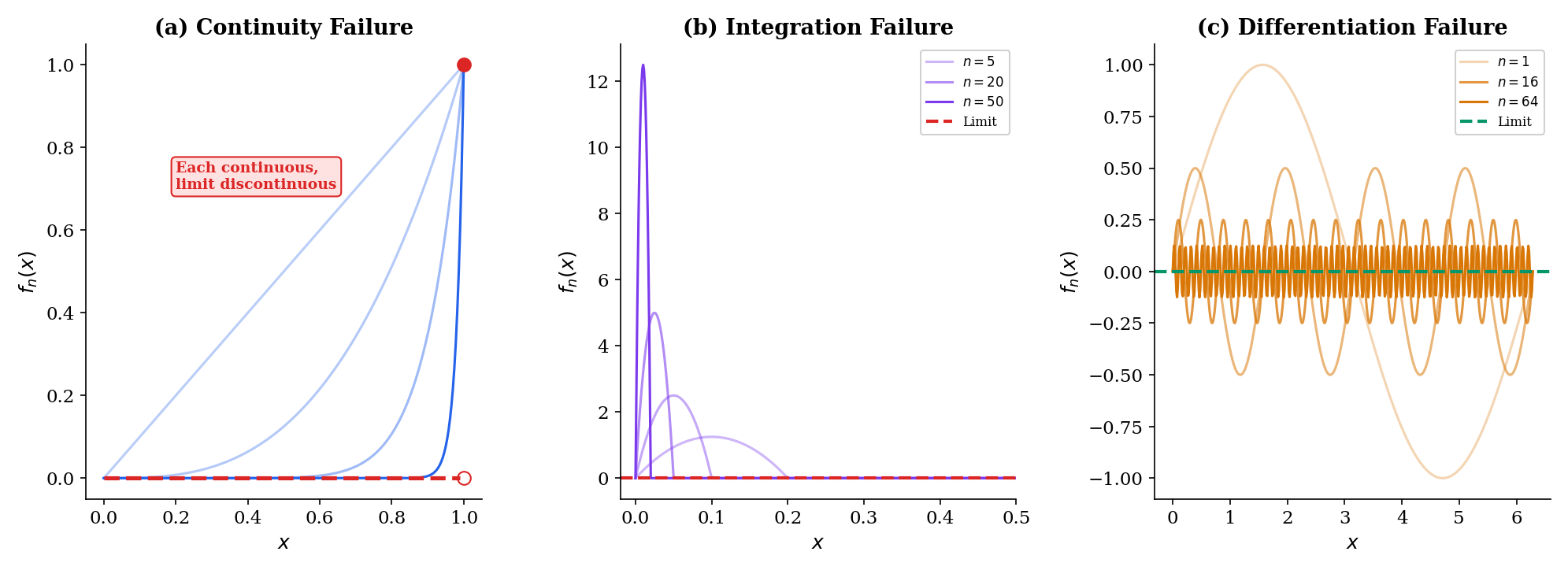
1. Continuity failure. We’ve just seen this: is continuous for every , but pointwise where is discontinuous. The limit of continuous functions need not be continuous under pointwise convergence.
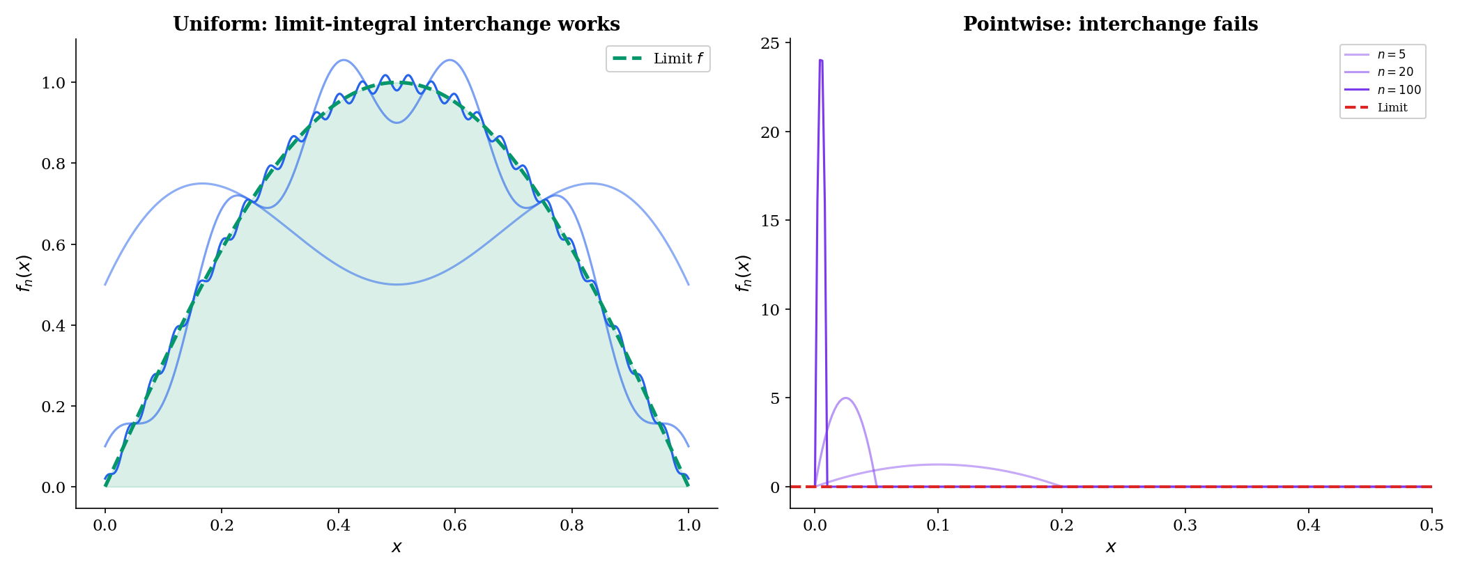
2. Integration failure. Consider the “moving bump” sequence on . Each has a bump near that grows taller and narrower. One can verify that as . But for each fixed (and ), so the pointwise limit is , and . We get
The limit and integral do not commute.
3. Differentiation failure. Let on . Then uniformly, so everywhere. But , and . The derivatives of the don’t converge at all, even though the themselves converge nicely.
💡 Remark 1
These three failures are not pathological edge cases. They arise naturally whenever convergence is “fast in some places and slow in others,” which is typical in machine learning: a neural network may fit training data well in dense regions and poorly in sparse regions, so the convergence of to is inherently non-uniform across the input domain. The distinction between pointwise and uniform convergence is the mathematical formalization of this problem.
Uniform Convergence — The Fix
If we require the convergence rate to be the same at every — that is, the depends only on , not on — then all three pathologies disappear.
📐 Definition 2 (Uniform Convergence)
A sequence of functions converges uniformly to on if for every , there exists such that
Equivalently, as .
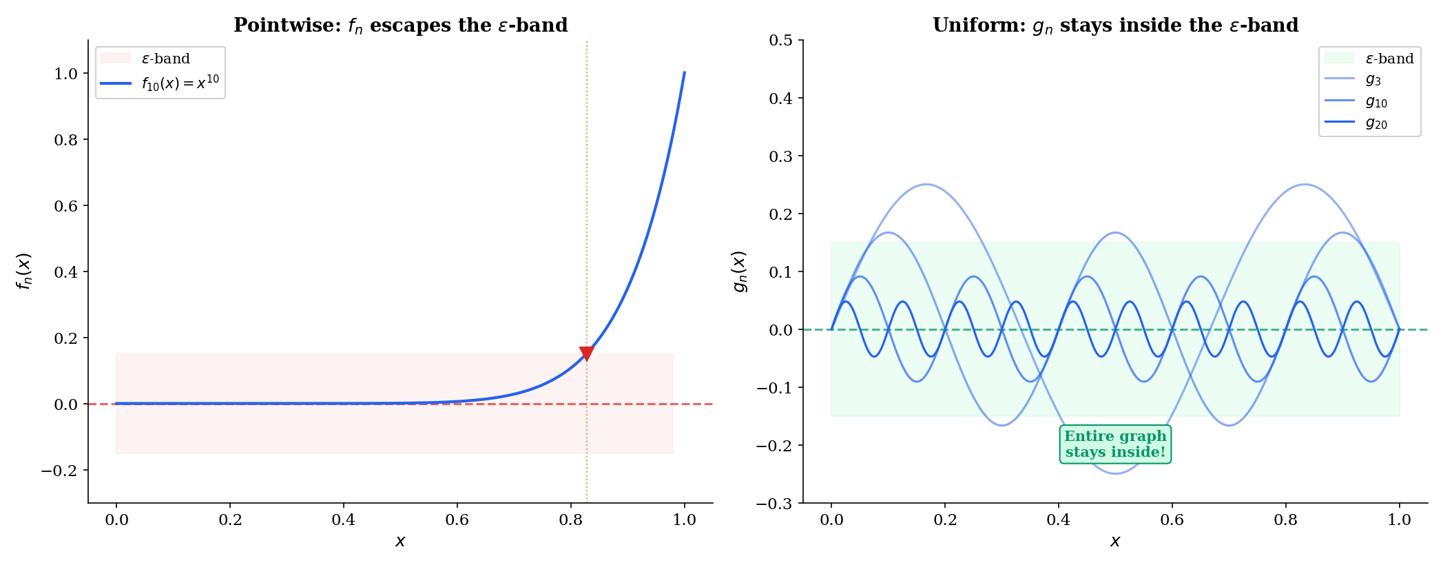
The geometric picture is the ε-band characterization: uniformly if and only if for every , eventually the entire graph of lies within an -band around the graph of . Not just at each point separately, but everywhere at once.
📐 Definition 3 (Sup-Norm / Uniform Metric)
For bounded functions , the sup-norm (or uniform norm) is
This is a genuine metric on the space of bounded functions on . Uniform convergence is convergence in this metric.
The comparison is now sharp:
- Pointwise: “for each , the vertical distance .”
- Uniform: “the maximum vertical distance over all simultaneously .”
🔷 Proposition 1 (Uniform ⟹ Pointwise)
If uniformly on , then pointwise on . The converse is false.
Proof.
If for , then in particular for each fixed , so .
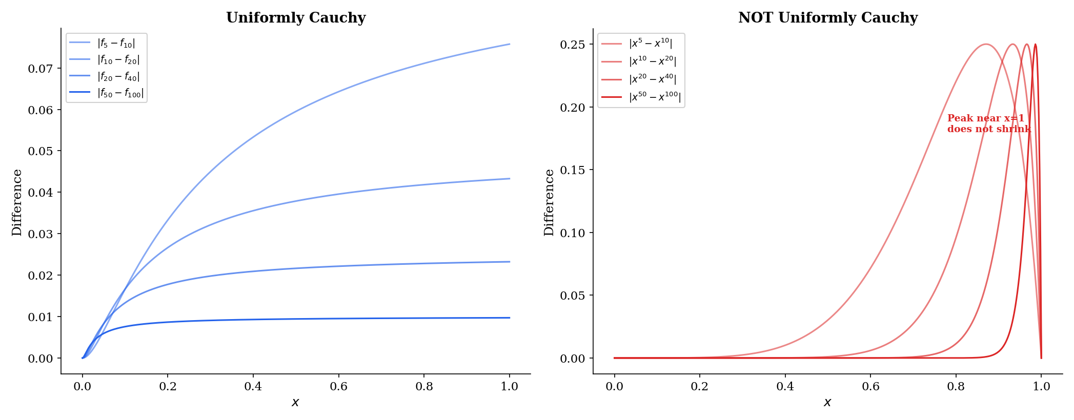
The converse fails: on converges pointwise but not uniformly — the sup-norm does not tend to because for any , we can find close to with close to .
📝 Example 2
on . Then , so uniformly. Compare with , where approaches , not .
Use the explorer below to feel the difference. Drag the slider and watch whether the function’s graph stays inside the ε-band. The moment when escapes the band near — but stays inside — is the difference between pointwise and uniform convergence.
||f_n - f||_∞ → 1 (never → 0) · Analogous to an overfit model converging fast in-distribution but failing at the boundary.
The Uniform Limit Theorem
The most important theorem in this topic: uniform convergence preserves continuity.
🔷 Theorem 1 (Uniform Limit Theorem)
If each is continuous at and uniformly on , then is continuous at .
Proof.
Fix . We need such that . Apply the triangle inequality:
Step 1 (Uniform convergence). Choose such that . Then for all , and .
Step 2 (Continuity of ). Since is continuous at , choose such that .
Step 3 (Combine). For :
The key insight: uniform convergence provides a single that simultaneously controls the first and third terms for all . Pointwise convergence would give different for different , and we couldn’t fix before choosing .
💡 Remark 2
The ε/3 trick is a paradigm: when bounding through an intermediary , split the triangle inequality into three terms and allocate to each. This proof strategy recurs throughout analysis — and in ML, it appears in decomposing generalization error into approximation error + estimation error + optimization error, each bounded by .
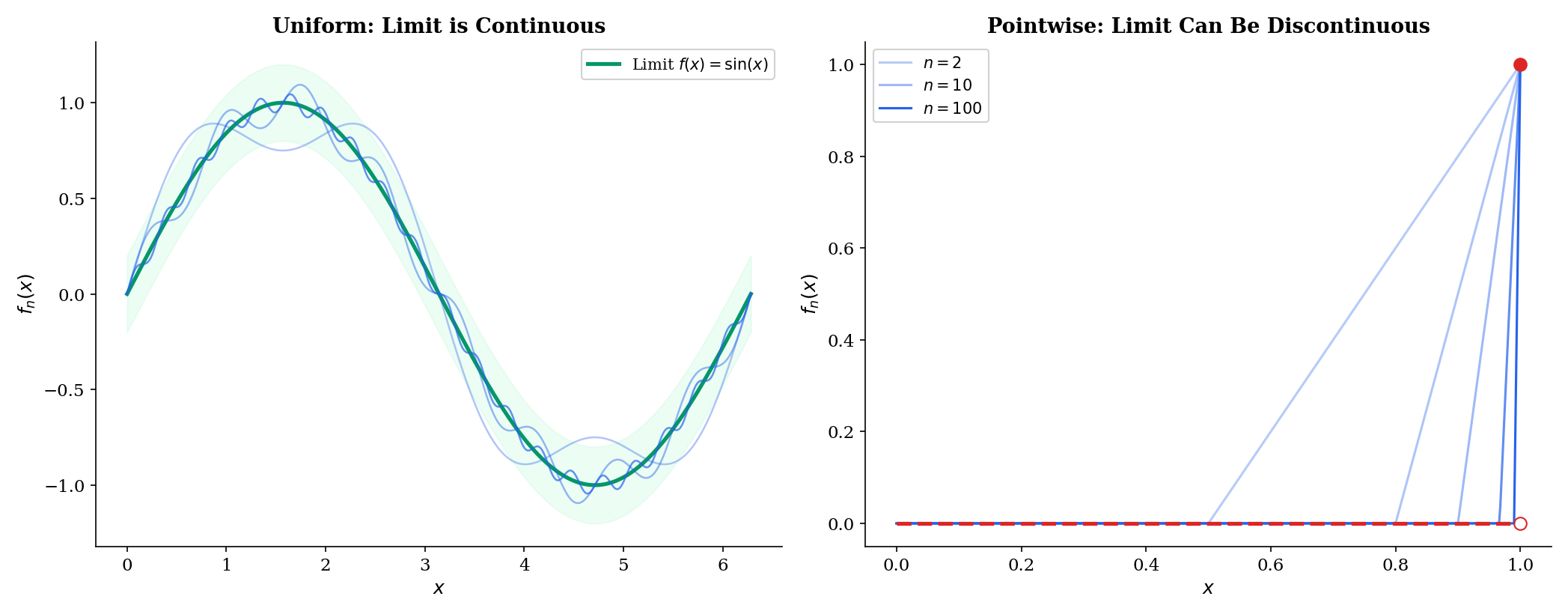
Uniform convergence (x^n/n → 0): the limit is continuous. The ε/3 argument works because one N controls all x.
Interchange Theorems — Integration and Differentiation
Uniform convergence enables two crucial interchange theorems, but with different hypotheses.
🔷 Theorem 2 (Interchange of Limit and Integral)
If uniformly on and each is Riemann integrable on , then is Riemann integrable and
Proof.
Since by uniform convergence, the right side tends to .
The proof is clean and direct — the sup-norm bound converts a pointwise inequality into a uniform one, and the integral of a uniform bound is just the bound times the interval length.
📝 Example 3
The interchange fails for pointwise convergence. Our “moving bump” sequence has for all but pointwise, so .
The differentiation interchange is harder and requires a stronger hypothesis:
🔷 Theorem 3 (Interchange of Limit and Derivative)
If is a sequence of differentiable functions on such that:
(i) for at least one , and
(ii) uniformly on ,
then uniformly for some differentiable , and .
💡 Remark 3
The differentiation interchange requires uniform convergence of the derivatives, not the functions themselves. This asymmetry is fundamental: integration is a smoothing operation (it improves convergence), while differentiation is a roughening operation (it can destroy convergence). In ML terms: backpropagation computes derivatives, so uniform convergence of loss landscapes does not automatically imply well-behaved gradients .
The Cauchy Criterion for Uniform Convergence
Just as numerical sequences have a Cauchy criterion that certifies convergence without knowing the limit (Sequences, Limits & Convergence, Definition 6), function sequences have an analogous criterion.
🔷 Proposition 2 (Cauchy Criterion for Uniform Convergence)
A sequence converges uniformly on if and only if for every , there exists such that
Proof.
(⟹) If uniformly, then . Given , choose such that for . Then for .
(⟸) For each fixed , the numerical sequence satisfies , so is Cauchy in . By completeness of (from Completeness & Compactness), for some value .
To show the convergence is uniform: fix and choose from the hypothesis. For any and any , . Taking gives for all , which is .
💡 Remark 4
The Cauchy criterion shows that with the sup-norm is a complete space — every uniformly Cauchy sequence of continuous functions converges uniformly to a continuous function. This completeness is the function-space analog of the completeness of from Completeness & Compactness. It will be formalized as a Banach space structure in Normed & Banach Spaces.
Series of Functions and the Weierstrass M-Test
A series of functions is just a sequence of partial sums. The Weierstrass M-test provides a practical, checkable criterion for uniform convergence.
📐 Definition 4 (Uniform Convergence of a Series)
A series converges uniformly on if the sequence of partial sums converges uniformly on .
🔷 Theorem 4 (Weierstrass M-Test)
Let and suppose there exist constants such that for all and all . If converges, then converges uniformly (and absolutely) on .
Proof.
For :
Since converges, its tail , so is uniformly Cauchy. By the Cauchy criterion (Proposition 2), converges uniformly.
📝 Example 4
The series converges uniformly on . Take ; since and , the M-test applies. Since each is continuous and the convergence is uniform, the Uniform Limit Theorem (applied to partial sums) guarantees the sum defines a continuous function.
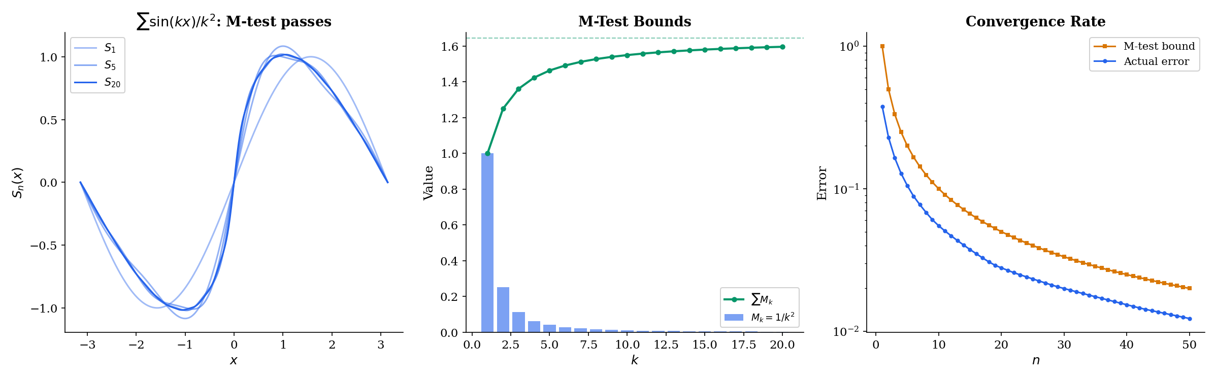
M_k = 1/k² (∑ = π²/6) · Left: partial sums S_n(x) vs. full sum. Right: M_k bound bars (blue = included, gray = tail).
Equicontinuity and the Arzelà-Ascoli Theorem
The Heine-Borel theorem from Completeness & Compactness says that a subset of is compact if and only if it is closed and bounded. What is the analog for subsets of the function space ? Boundedness alone is not enough — we need a condition that controls how much the functions in the family can oscillate. That condition is equicontinuity.
📐 Definition 5 (Equicontinuity)
A family of functions is equicontinuous if for every , there exists such that
Compare this with uniform continuity from Epsilon-Delta & Continuity (Definition 9): uniform continuity says a single function has one that works at every point; equicontinuity says a family of functions has one that works for every function and every point simultaneously.
📐 Definition 6 (Pointwise Boundedness)
A family is pointwise bounded if for each , .
🔷 Theorem 5 (Arzelà-Ascoli Theorem)
A subset is relatively compact (every sequence in has a uniformly convergent subsequence) if and only if is equicontinuous and pointwise bounded.
Proof.
(⟸, main direction.) Let .
Step 1 (Diagonal extraction on the rationals). Let be an enumeration of the rationals in . By pointwise boundedness, is a bounded sequence in , so by the Bolzano-Weierstrass theorem (Sequences, Limits & Convergence, Theorem 4), we can extract a subsequence that converges at . From that subsequence, extract a further subsequence converging at . Continue. The diagonal subsequence — the -th term of the -th subsequence — converges at every rational .
Step 2 (Extend from rationals to all of ). By equicontinuity, for any , choose from the definition. For any , find a rational with . Then for indices in our diagonal subsequence:
for sufficiently large. The first and third terms use equicontinuity ( works for all ); the middle term uses convergence at .
Step 3 (Convergence is uniform). The same from equicontinuity works at every , so the bound above is independent of . This gives , so the diagonal subsequence is uniformly Cauchy and hence uniformly convergent.
(⟹, sketch.) If is relatively compact, a finite -net argument shows equicontinuity: cover with finitely many -balls, use the uniform continuity of each center function, and take the minimum . Pointwise boundedness follows similarly.
💡 Remark 5
The Arzelà-Ascoli proof uses the same diagonal argument that appears in Cantor’s proof and in many ML contexts — extracting convergent subsequences from parameter sequences in optimization. The equicontinuity condition has a direct ML interpretation: a family of neural networks with bounded Lipschitz constants (achieved by spectral normalization or gradient clipping) is equicontinuous, and Arzelà-Ascoli guarantees a convergent subsequence — the function-space analog of compactness in parameter space.
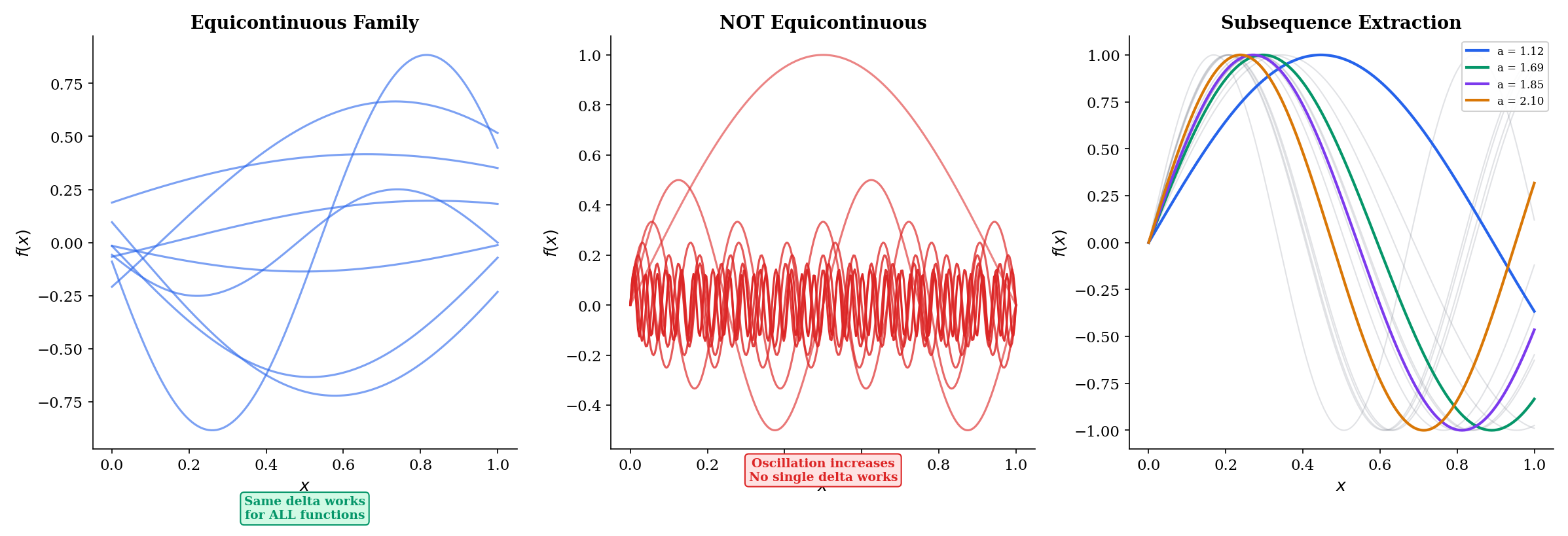
Click on the graph to probe equicontinuity at a point. Blue curves = extracted subsequence. Dashed red = limit approximation.
Connections to Statistics
Uniform convergence is the foundation of empirical-process theory and of every consistency result for M-estimators in statistics.
Glivenko–Cantelli and Donsker
The Glivenko–Cantelli theorem is the canonical uniform Law of Large Numbers — the empirical CDF converges uniformly to the true CDF. Donsker’s theorem lifts this to a CLT-style statement uniform over function classes. The pointwise-vs-uniform distinction developed here is the entire foundation of empirical-process theory. See formalStatistics Empirical Processes.
Bootstrap validity
Bootstrap consistency rests on Glivenko–Cantelli: the bootstrap samples from , and uniform closeness of to underwrites the consistency of bootstrap estimates. Without uniform convergence, bootstrap distributions could agree pointwise with the truth yet miss it sup-norm-wise — exactly the kind of gap GC closes. See formalStatistics Bootstrap.
M-estimator consistency
The Uniform LLN over a parameter set is required for consistency of M-estimators: converges to only when uniformly. This is precisely why textbooks insist on uniform — not pointwise — convergence in the consistency theorem for the MLE. See formalStatistics Law of Large Numbers.
Connections to ML
Uniform convergence is not merely a theoretical curiosity that happens to appear in machine learning. It is the mathematical foundation of generalization theory — the question of why models that perform well on training data also perform well on unseen data.
Uniform convergence of empirical processes
Given a hypothesis class (e.g., the set of all neural networks with a fixed architecture), the empirical risk of a hypothesis on training examples is
while the true risk is . The law of large numbers guarantees that for any fixed , as . This is pointwise convergence — one hypothesis at a time.
But learning requires more: we need to be close to for all simultaneously, so that the hypothesis that minimizes also approximately minimizes . This is uniform convergence:
This is exactly the sup-norm over the function class . → formalML PAC Learning
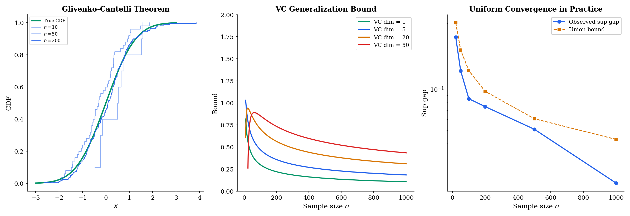
The Glivenko-Cantelli theorem
The oldest and most fundamental uniform convergence result in statistics: the empirical CDF converges uniformly to the true CDF :
The Dvoretzky-Kiefer-Wolfowitz (DKW) inequality gives the rate: , yielding . The Kolmogorov-Smirnov test is built on this sup-norm. → formalML Concentration Inequalities
VC dimension and complexity control
The VC dimension of a hypothesis class quantifies how “complex” is — it is the largest number of points that can shatter (classify in all possible ways). The fundamental theorem of statistical learning: is PAC-learnable if and only if has finite VC dimension. The generalization bound
is a rate of uniform convergence — it tells you how fast the sup-norm between empirical and true risk shrinks with sample size. → formalML PAC Learning
Arzelà-Ascoli and neural network approximation
The universal approximation theorem says that neural networks are dense in under the sup-norm: for any continuous and any , there exists a neural network with . Arzelà-Ascoli constrains which families of networks are compact (and hence tractable): a family with bounded Lipschitz constants is equicontinuous, and equicontinuity + boundedness gives compactness. This is why Lipschitz constraints (spectral normalization, gradient penalty) appear in generative models — they enforce the compactness that makes optimization well-posed.
Computational Notes
Uniform convergence can be verified computationally by evaluating the sup-norm on a dense grid.
Computing the sup-norm. Given a function sequence and its limit , we approximate by sampling:
import numpy as np

def sup_norm(fn, f, domain, grid_size=1000):
    """Approximate ||fn - f||_∞ on domain."""
    x = np.linspace(domain[0], domain[1], grid_size)
    return np.max(np.abs(fn(x) - f(x)))

# x^n on [0, 1]: not uniform (sup norm → 1)
for n in [10, 50, 100, 500]:
    fn = lambda x, n=n: x**n
    f = lambda x: np.where(x < 1, 0.0, 1.0)
    print(f"n={n:3d}: ||f_n - f||_∞ = {sup_norm(fn, f, (0, 1)):.6f}")

# x^n/n on [0, 1]: uniform (sup norm = 1/n → 0)
for n in [10, 50, 100, 500]:
    gn = lambda x, n=n: x**n / n
    g = lambda x: np.zeros_like(x)
    print(f"n={n:3d}: ||g_n - g||_∞ = {sup_norm(gn, g, (0, 1)):.6f}")
Verifying the integration interchange. Compare with :
from scipy import integrate

def check_interchange(fn, f, domain, n_values):
    """Compare lim ∫f_n with ∫(lim f_n)."""
    a, b = domain
    integral_f = integrate.quad(f, a, b)[0]
    for n in n_values:
        integral_fn = integrate.quad(lambda x: fn(x, n), a, b)[0]
        print(f"n={n:3d}: ∫f_n = {integral_fn:.6f}, ∫f = {integral_f:.6f}, "
              f"gap = {abs(integral_fn - integral_f):.6f}")

# Uniform case: gap → 0
check_interchange(
    fn=lambda x, n: x**n / n,
    f=lambda x: 0.0,
    domain=(0, 1),
    n_values=[5, 20, 100]
)
Implementing the Weierstrass M-test. Check the bound and compare with the actual tail error:
def weierstrass_m_test(term, Mk, domain, n_terms, max_k=200, grid=1000):
    """Apply the M-test: compare actual tail error with M-bound."""
    x = np.linspace(domain[0], domain[1], grid)
    partial = sum(term(x, k) for k in range(1, n_terms + 1))
    full = sum(term(x, k) for k in range(1, max_k + 1))
    actual_error = np.max(np.abs(full - partial))
    m_bound = sum(Mk(k) for k in range(n_terms + 1, max_k + 1))
    print(f"n={n_terms}: actual ||S-S_n||_∞ = {actual_error:.6f}, "
          f"M-bound = {m_bound:.6f}")

# ∑ sin(kx)/k²
weierstrass_m_test(
    term=lambda x, k: np.sin(k * x) / k**2,
    Mk=lambda k: 1 / k**2,
    domain=(0, 2 * np.pi),
    n_terms=10
)
Computing the Kolmogorov-Smirnov statistic. The sup-norm between empirical and true CDF:
def kolmogorov_smirnov(samples, cdf):
    """Compute ||F_hat_n - F||_∞."""
    n = len(samples)
    sorted_samples = np.sort(samples)
    ecdf = np.arange(1, n + 1) / n
    sup_diff = np.max(np.abs(ecdf - cdf(sorted_samples)))
    return sup_diff

# Standard normal: Glivenko-Cantelli in action
from scipy.stats import norm
for n in [100, 1000, 10000]:
    samples = np.random.randn(n)
    ks = kolmogorov_smirnov(samples, norm.cdf)
    dkw_bound = np.sqrt(np.log(2 / 0.05) / (2 * n))
    print(f"n={n:5d}: KS = {ks:.4f}, DKW 95% bound = {dkw_bound:.4f}")
Connections & Further Reading
Prerequisites — topics you need first
Sequences, Limits & Convergence
Pointwise and uniform convergence of function sequences extend the epsilon-N convergence of numerical sequences from Topic 1. The Cauchy criterion for uniform convergence is the function-space analog of the Cauchy criterion for sequences. Convergence rates (sublinear, linear, quadratic) reappear as rates of uniform convergence over function classes.
Epsilon-Delta & Continuity
The Uniform Limit Theorem proves that uniform convergence preserves continuity — the epsilon-delta framework from Topic 2 is the tool used in the proof (the epsilon/3 argument). Uniform continuity and Lipschitz continuity from Topic 2 reappear in the equicontinuity condition of the Arzela-Ascoli theorem.
Completeness & Compactness
The Arzela-Ascoli theorem is a compactness result in function space C([a,b]), extending the Heine-Borel theorem from R^n. Equicontinuity + pointwise boundedness plays the role that closed + bounded plays in Heine-Borel. Completeness of R under the sup-norm means that uniformly Cauchy sequences converge.
Where this leads — next in formalCalculus
Series Convergence & Tests
Power Series & Taylor Series
Fourier Series & Orthogonal Expansions
Approximation Theory
Metric Spaces & Topology
On to formalStatistics — where this calculus powers inference
Empirical Processes
Glivenko–Cantelli (sup_x |F_n(x) - F(x)| →_a.s. 0) is the canonical uniform LLN. Donsker's theorem lifts this to a CLT uniform over function classes. The pointwise-vs-uniform distinction is the foundation of the entire field.
Bootstrap
Bootstrap validity rests on Glivenko–Cantelli — uniform convergence of F_n to F. The bootstrap samples from F_n, and uniform closeness of F_n to F underwrites the consistency of bootstrap estimates.
Law Of Large Numbers
The Uniform LLN (uniform over a parameter θ ∈ Θ) is required for consistency of M-estimators: θ̂_n = argmin M_n(θ) converges to argmin M(θ) only when M_n → M uniformly.
On to formalML — where this calculus powers ML
PAC Learning
PAC learning is fundamentally a uniform convergence result: the empirical risk R_hat_n(h) converges uniformly to the true risk R(h) over the hypothesis class H as the sample size n grows. The VC dimension quantifies the complexity of H and controls the rate of uniform convergence — larger VC dimension means slower convergence and more data required for generalization.
Concentration Inequalities
Uniform convergence bounds like the Glivenko-Cantelli theorem and the Dvoretzky-Kiefer-Wolfowitz inequality are concentration inequalities applied uniformly over function classes. The DKW inequality bounds ||F_hat_n - F||_infinity — the sup-norm distance between empirical and true CDFs — at rate O(1/sqrt(n)).
Measure Theoretic Probability
Modes of convergence in probability — almost sure convergence, convergence in probability, convergence in distribution — extend the pointwise/uniform distinction from deterministic function sequences to sequences of random variables. Uniform integrability, the probabilistic analog of equicontinuity, controls interchange of limits and expectations.
References
- book Abbott (2015). Understanding Analysis Chapter 6 develops uniform convergence with the epsilon-band characterization and proves the Uniform Limit Theorem — the primary reference for our geometric-first approach
- book Rudin (1976). Principles of Mathematical Analysis Chapter 7 on sequences and series of functions — the definitive treatment of uniform convergence, the Weierstrass M-test, and equicontinuity
- book Tao (2016). Analysis I Chapter 14 on uniform convergence — careful first-principles development distinguishing pointwise and uniform convergence at every step
- book Kreyszig (1989). Functional Analysis Chapter 1 on normed spaces and Chapter 5 on compact operators — the sup-norm as a genuine norm on C([a,b]) and Arzela-Ascoli as a compactness criterion
- book Shalev-Shwartz & Ben-David (2014). Understanding Machine Learning: From Theory to Algorithms Chapters 4-6 develop PAC learning and VC dimension as uniform convergence results over hypothesis classes — the direct ML application of the theory developed here
- paper Vapnik & Chervonenkis (1971). “On the Uniform Convergence of Relative Frequencies of Events to Their Probabilities” The foundational paper introducing VC dimension and establishing the connection between uniform convergence and learnability