Normed & Banach Spaces
Adding algebraic structure to metric spaces — from norms and bounded linear operators through the Baire Category Theorem to the three pillars of functional analysis, with applications to spectral normalization, dual-space optimization, and generalization bounds.
Abstract. A metric space tells you how far apart points are. A normed space tells you how far apart points are using a notion of length that respects the vector space structure — addition and scalar multiplication. When a normed space is complete (every Cauchy sequence converges), it is a Banach space, and a remarkable trio of theorems becomes available. The Baire Category Theorem — a complete metric space cannot be 'thin' — is the engine behind three pillars of linear functional analysis: the Uniform Boundedness Principle (pointwise-bounded families of operators are uniformly bounded), the Open Mapping Theorem (surjective bounded operators between Banach spaces map open sets to open sets), and the Closed Graph Theorem (a closed-graph linear operator between Banach spaces is automatically bounded). These are not abstract curiosities. The operator norm controls Lipschitz constants of neural network layers — spectral normalization enforces this directly. Dual spaces and bounded linear functionals power Fenchel conjugates and mirror descent. The Uniform Boundedness Principle underlies generalization bounds in statistical learning. This topic builds the Banach space infrastructure that modern optimization theory and machine learning assume.
1. Overview and Motivation
Consider a single layer of a neural network: , where is a weight matrix and is a bias vector. This map takes an input vector and produces an output vector — it is a linear operator between two vector spaces. The question that spectral normalization asks is: how much can this layer stretch its input? That stretching factor is the operator norm , and controlling it is essential for stable GAN training.
To make this precise, we need more than the metric-space framework from Topic 29. A metric tells us distances, but it does not know about addition or scalar multiplication — we cannot ask “how does stretch vectors?” in a plain metric space, because there are no vectors to stretch. We need a normed space: a vector space equipped with a notion of length (a norm) that interacts with the algebraic operations. When that normed space is also complete — every Cauchy sequence converges — we have a Banach space, and a remarkable collection of theorems becomes available.
The arc of this topic follows a natural staircase of structure:
- Normed spaces (Section 2): vector spaces with a notion of length.
- Banach spaces (Section 4): complete normed spaces — the “good” spaces where analysis works.
- Bounded linear operators (Section 5): the morphisms that respect both the algebraic and metric structure.
- The Baire Category Theorem (Section 6): the deep consequence of completeness that powers everything.
- The three pillars (Sections 7–9): Uniform Boundedness, Open Mapping, Closed Graph — all consequences of Baire, all load-bearing in functional analysis.
- Dual spaces (Section 10): the space of bounded linear functionals, where optimization lives.
This is the second topic in Track 8 (Functional Analysis Essentials). Topic 29 built the metric infrastructure — completeness, compactness, the Banach fixed-point theorem, Arzelà–Ascoli. Topic 30 adds algebra: metric + vector space = Banach space, and the algebraic compatibility unlocks theorems that have no analog in plain metric spaces.
2. Normed Vector Spaces
📐 Definition 1 (Normed Vector Space)
A normed vector space (or normed space) is a pair where is a vector space over (or ) and satisfies:
- Positive definiteness: if and only if .
- Absolute homogeneity: for all scalars and all .
- Triangle inequality: for all .
Every norm induces a metric . This metric is translation-invariant () and absolutely homogeneous () — properties that a general metric need not have.
The key insight: a norm carries more information than a metric. It knows about the vector-space structure. This algebraic compatibility is what makes bounded linear operators and dual spaces possible.
📝 Example 1 (ℝⁿ with ℓᵖ Norms)
For , the norm on is:
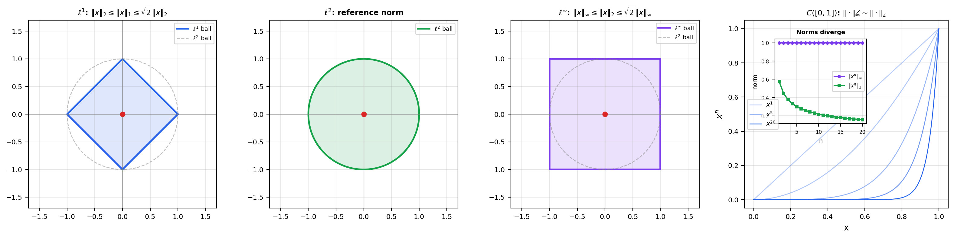
with . Each gives a valid normed space. The unit balls change shape: a diamond for , a circle for , a square for . All three norms are equivalent on (Theorem 1 below), but this equivalence fails spectacularly in infinite dimensions.
📝 Example 2 (C([a,b]) with the Sup-Norm)
The space of continuous functions on with is a normed space. Topic 29 (Theorem 2) proved that this space is complete under this norm — it is our first infinite-dimensional Banach space.
📝 Example 3 (Lᵖ(μ) Spaces)
💡 Remark 1 (Lᵖ Vocabulary Refresh)
If you completed Track 7 (Topics 25–28) some time ago, here is a quick refresher. consists of (equivalence classes of) measurable functions with finite . The key results we will cite: Hölder’s inequality with (Topic 27, Theorem 2), the Riesz-Fischer completeness theorem (Topic 27, Theorem 5), and the duality (Topic 27, Theorem 8; full proof via Radon-Nikodym in Topic 28).
📝 Example 4 (ℓᵖ Sequence Spaces)
The discrete analog of : with . These are spaces over . They are simpler to compute with and serve as test cases for every abstract theorem in this topic.
3. Equivalence of Norms in Finite Dimensions
In , all norms are equivalent — they induce the same topology, the same convergent sequences, the same Cauchy sequences. This is a finite-dimensional luxury that fails dramatically in infinite dimensions.
🔷 Theorem 1 (Equivalence of Norms on ℝⁿ)
Any two norms and on are equivalent: there exist constants such that:
Consequently, all norms on induce the same open sets, the same convergent sequences, and the same Cauchy sequences. Completeness, compactness, and continuity are norm-independent in finite dimensions.
Proof.
It suffices to show every norm on is equivalent to .
Upper bound. Let be the standard basis. For :
By Cauchy-Schwarz:
where .
Lower bound. The function is continuous in the topology (by the upper bound and the reverse triangle inequality). The unit sphere is compact in (Heine-Borel, Topic 3). By the extreme value theorem, attains a minimum on . Then for :
💡 Remark 2 (Infinite-Dimensional Failure)
On , the and norms are NOT equivalent. The sequence satisfies for all , but . No constant satisfies for all . The proof above fails because the unit sphere in infinite dimensions is NOT compact (Topic 29, Example 8).
4. Banach Spaces
📐 Definition 2 (Banach Space)
A Banach space is a complete normed vector space — a normed space in which every Cauchy sequence converges (in the norm).
Equivalently: is a complete metric space under the metric induced by the norm.
The following characterization is often more convenient in practice than the Cauchy-sequence definition.
🔷 Proposition 1 (Absolute Convergence Implies Convergence)
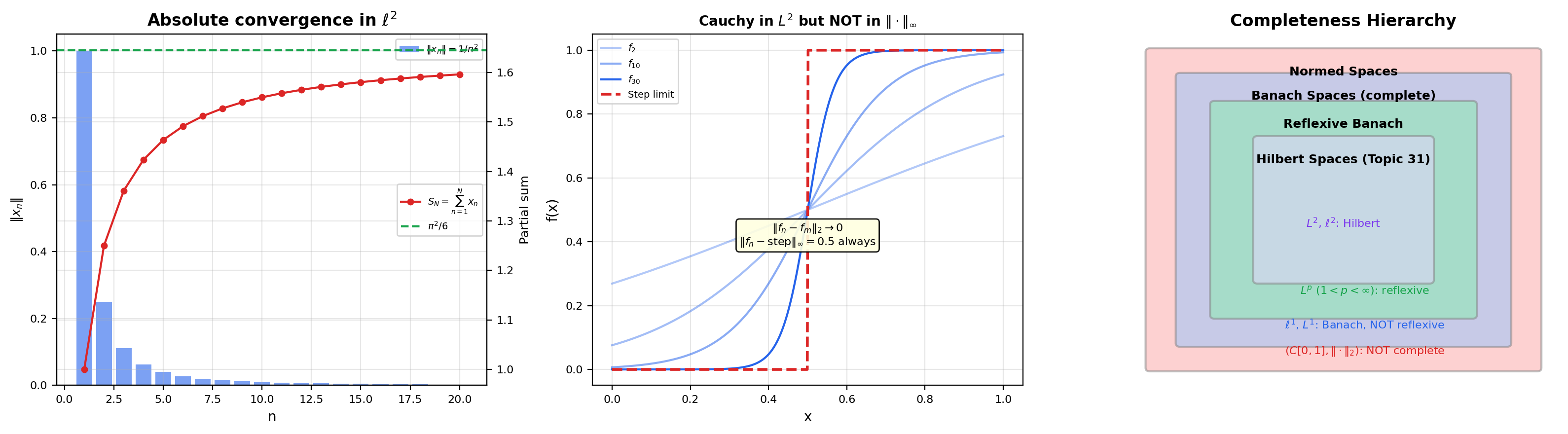
A normed space is a Banach space if and only if every absolutely convergent series converges: whenever , the partial sums converge in .
Proof.
() If , then for :
as , so is Cauchy. By completeness, converges.
() Let be Cauchy. Choose a subsequence with . Then satisfies . By hypothesis, converges, so the telescoping partial sums , giving . Since is Cauchy with a convergent subsequence, .
📝 Example 5 (Catalog of Banach Spaces)
The reader has already seen these completeness results. Collected here for reference:
- with any norm — complete (Bolzano-Weierstrass, Topic 3).
- with — complete (Topic 29, Theorem 2). A uniform limit of continuous functions is continuous.
- for — complete (Riesz-Fischer, Topic 27, Theorem 5).
- for — complete (special case of over counting measure).
- with — NOT complete (Topic 29, Example 7). Cauchy sequences of continuous functions can converge to a discontinuous function.
5. Bounded Linear Operators
📐 Definition 3 (Bounded Linear Operator)
Let and be normed spaces. A linear map is bounded if there exists such that for all .
For linear maps, bounded continuous continuous at one point. (The equivalence uses linearity to transfer local behavior to global behavior — a property that nonlinear maps do not enjoy.)
📐 Definition 4 (Operator Norm)
The operator norm of a bounded linear operator is:
All three expressions are equal. The operator norm is the smallest constant such that for all .
🔷 Theorem 2 (𝓑(X, Y) Is a Banach Space)
Let be a normed space and a Banach space. The space of bounded linear operators from to , equipped with the operator norm, is a Banach space.
In particular, the dual space is always a Banach space, regardless of whether itself is complete.
Proof.
Let be Cauchy in . For each :
So is Cauchy in . Since is Banach, define .
is linear: .
is bounded: Since is Cauchy, it is bounded: for some . Then .
in operator norm: Fix . Choose such that for . For any with :
Letting : . Since this holds for all , we get for .
📝 Example 6 (Operator Norm of a Matrix)
For viewed as :
- (maximum absolute column sum).
- (maximum absolute row sum).
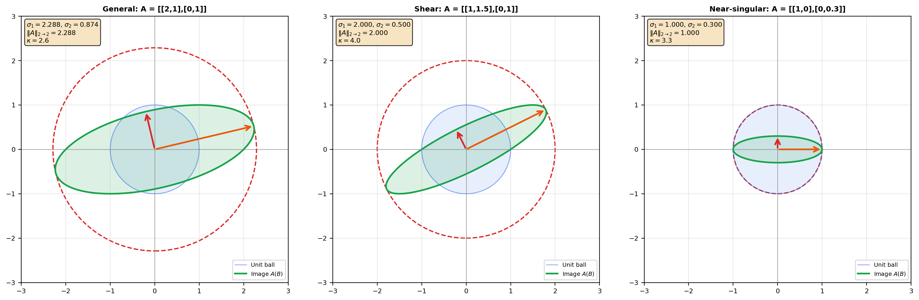
- (largest singular value). This is the spectral norm used in spectral normalization of neural networks.
An upper-triangular matrix with distinct singular values. Shows how the operator norm captures the worst-case stretch.
6. The Baire Category Theorem
We now prove the theorem that powers the three pillars of linear functional analysis. This was explicitly deferred from Topic 29 — it is a deep consequence of completeness that goes beyond the fixed-point machinery we developed there.
📐 Definition 5 (Nowhere Dense, Meager, and Residual Sets)
Let be a metric space.
- A set is nowhere dense if its closure has empty interior: . Equivalently, contains no open ball.
- A set is meager (or of the first category) if it is a countable union of nowhere-dense sets.
- A set is residual (or of the second category) if its complement is meager. Equivalently, it contains a countable intersection of open dense sets.
🔷 Theorem 3 (Baire Category Theorem)
Let be a complete metric space. Then is not meager in itself: cannot be written as a countable union of nowhere-dense sets.
Equivalently: if is a countable collection of open dense subsets of , then is dense in .
Proof.
We prove the “open dense” formulation. Let be open and dense in . We must show that is dense: for every nonempty open set , .
Construction. Since is dense and is open and nonempty, is nonempty and open. Choose and such that:
Since is dense and is open and nonempty, . Choose and with:
Inductively: choose and with:
Convergence. The sequence is Cauchy: for , , so . By completeness, for some .
Membership. For each : . Also . So .
💡 Remark 3 (Why Completeness Is Essential)
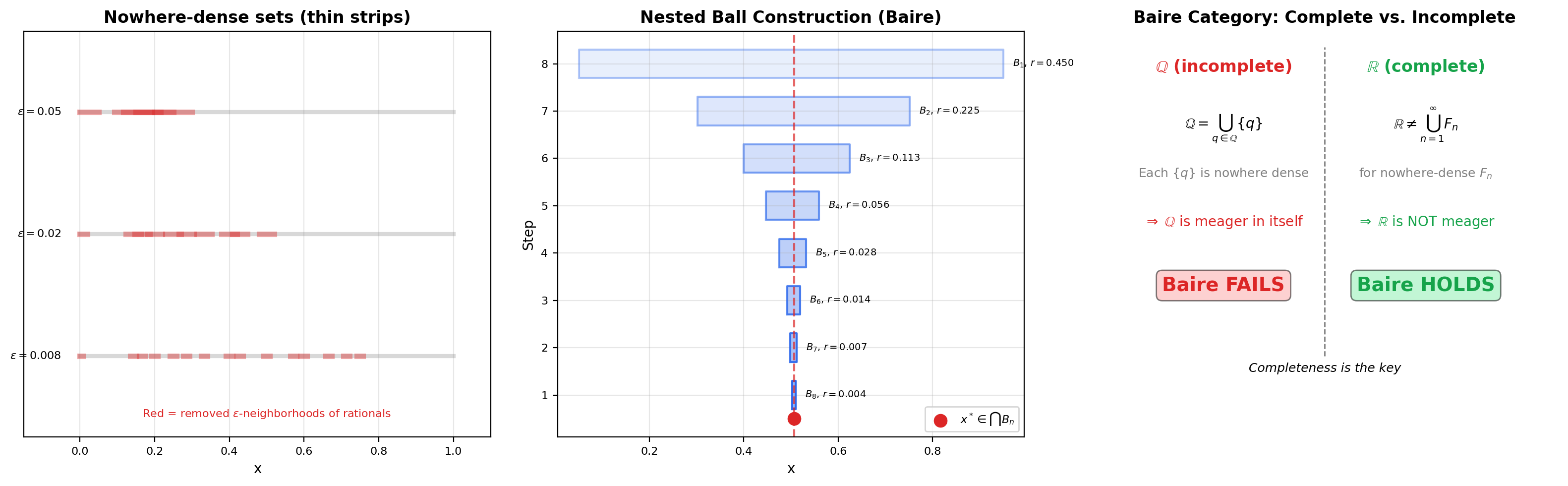
The rational numbers are a countable union of singletons , each nowhere dense. So is meager in itself. The Baire Category Theorem fails for because is not complete. Every application of Baire to Banach spaces relies on completeness — this is why we work in Banach spaces, not merely normed spaces.
📝 Example 7 (The Baire Category Theorem Applied to ℝ)
is complete, so it is not meager in itself. This means for any sequence of nowhere-dense sets . In particular, is uncountable — since every singleton is nowhere dense, this gives a proof of the uncountability of that does not use Cantor’s diagonal argument.
Remove thin intervals around rationals in [0,1] ⊂ ℝ. By Baire, the residual set is dense — the intersection of the complements is never empty.
7. The Uniform Boundedness Principle
The first consequence of Baire. This closes the deferral from Topic 29, Definition 16 (uniform boundedness of a family of operators).
🔷 Theorem 4 (Uniform Boundedness Principle (Banach-Steinhaus))
Let be a Banach space, a normed space, and a family of bounded linear operators. If the family is pointwise bounded — that is, for every — then it is uniformly bounded:
Proof.
For each , define the closed set:
By pointwise boundedness, . By Baire (Theorem 3), since is a Banach space (complete), some has nonempty interior: there exist and with .
For any with : the point , so for all .
Then:
So for all , giving for all .
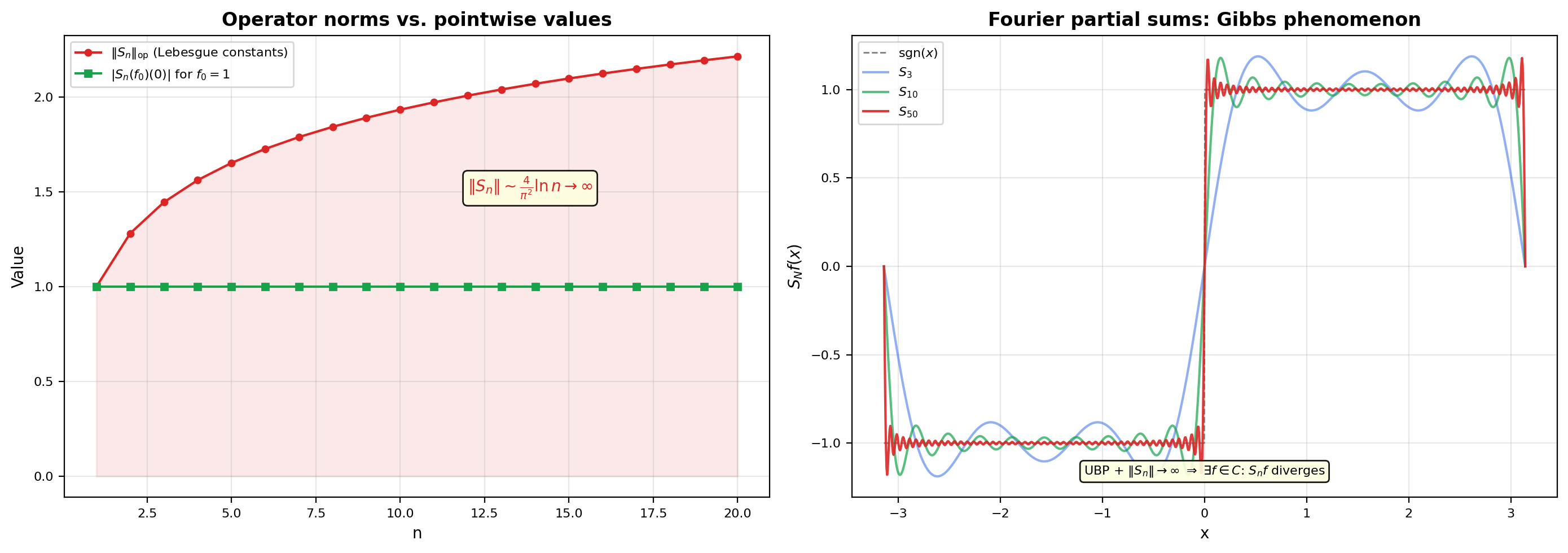
📝 Example 8 (Fourier Coefficients and Pointwise Convergence)
Consider the partial Fourier sum operators defined by . Each is a bounded linear functional. One can show (the Lebesgue constants grow logarithmically). By UBP, if converged for every , the operator norms would be uniformly bounded — but they are not. So there must exist a continuous function whose Fourier series diverges at 0 (du Bois-Reymond’s theorem). This is UBP as an existence tool: it proves the existence of a “bad” function without constructing one.
💡 Remark 4 (UBP and Generalization Bounds)
In statistical learning theory, a function class is “learnable” if empirical risk converges uniformly to population risk: . This is a uniform boundedness condition on the evaluation functionals restricted to . The UBP-style reasoning — “pointwise control implies uniform control” — is the conceptual template that PAC learning formalizes combinatorially via VC dimension.
8. The Open Mapping Theorem
The second consequence of Baire. Surjective bounded linear operators between Banach spaces map open sets to open sets — a result that is both surprising and immensely useful.
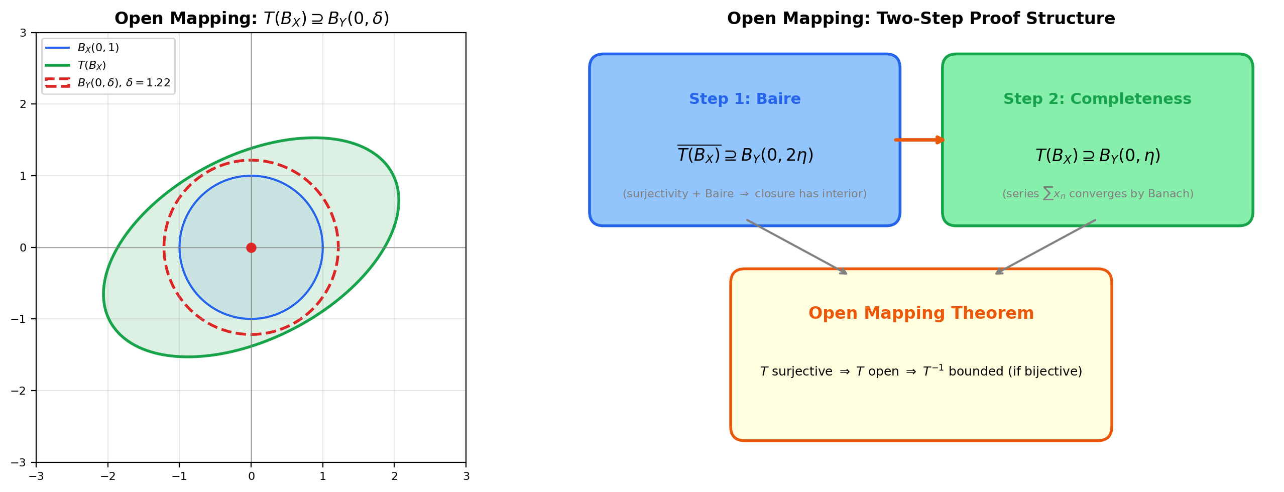
🔷 Theorem 5 (Open Mapping Theorem (Banach-Schauder))
Let and be Banach spaces and a surjective bounded linear operator. Then is an open mapping: is open in whenever is open in .
Equivalently: there exists such that — the image of the unit ball contains a ball.
Proof.
Step 1: The closure of contains a ball.
Since is surjective, . By Baire, some has nonempty interior. By scaling, has nonempty interior. Since the set is symmetric (if then ) and convex, it contains a ball centered at the origin:
Step 2: Upgrade from closure to itself.
We show . Take with . Since (by scaling), choose with and .
Then , so choose with and:
Inductively: and .
Since and is Banach, converges with , and .
🔷 Corollary 1 (Bounded Inverse Theorem)
If is a bounded linear bijection between Banach spaces, then is also bounded. That is, a bijective bounded linear operator between Banach spaces is an isomorphism.
Proof.
is surjective and bounded, so by the Open Mapping Theorem, is open. The inverse map maps open sets to open sets (the preimage under of an open set is , which is open). So is continuous, hence bounded.
9. The Closed Graph Theorem
The third consequence of Baire, proved via the Open Mapping Theorem.
📐 Definition 6 (Closed Graph)
A linear operator has a closed graph if the graph is closed in the product topology. Equivalently: whenever in and in , then .
🔷 Theorem 6 (Closed Graph Theorem)
Let and be Banach spaces and a linear operator. If has a closed graph, then is bounded.
Proof.
Define the product norm on . Since and are Banach spaces, is a Banach space.
The graph is a closed linear subspace of , hence itself a Banach space.
The projection defined by is bounded (with ), linear, and bijective (since is a function).
By the Bounded Inverse Theorem (Corollary 1), is bounded:
Then , so is bounded.
💡 Remark 5 (When to Use the Closed Graph Theorem)
The CGT is a verification tool: to check that an operator is bounded, show instead that its graph is closed (i.e., check the sequential criterion ). This is often easier than directly estimating . The CGT is used throughout PDE theory (to show that differential operators with appropriate domains are bounded) and in operator algebras.
📝 Example 9 (The Three Pillars in Action)
The three theorems have a logical dependency:
- Baire UBP (directly).
- Baire Open Mapping Theorem (directly).
- Open Mapping Bounded Inverse Theorem Closed Graph Theorem.
So the Baire Category Theorem is the single engine: completeness of the space, combined with the algebraic structure of linear operators, produces all three.
10. Dual Spaces and Bounded Linear Functionals
📐 Definition 7 (Dual Space)
The dual space of a normed space is — the Banach space of all bounded linear functionals , equipped with the operator norm:
By Theorem 2, is always a Banach space, even if is not complete.
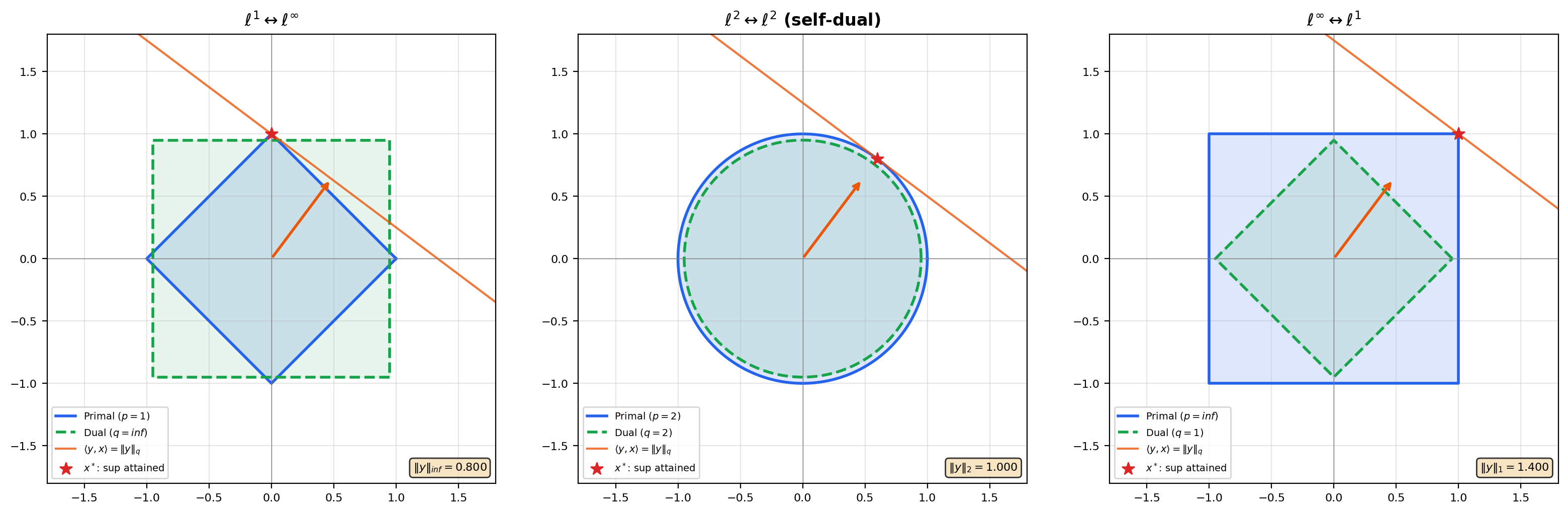
📝 Example 10 (Dual of ℓᵖ)
For , the dual of is where : every has the form for a unique , and .
Special cases:
- — self-dual (this foreshadows the Riesz representation in Topic 31).
- — bounded linear functionals on are identified with bounded sequences.
📝 Example 11 (Dual of Lᵖ)
Citing Topics 27–28. For and -finite : with (Topic 27, Theorem 8). The proof uses the Radon-Nikodym theorem (Topic 28) to represent the functional as .
(same proof structure). But is strictly larger than — it contains singular functionals (e.g., Banach limits) that are not representable as integrals. This asymmetry is why is “harder” to work with.
🔷 Theorem 7 (Hahn-Banach Extension Theorem (Statement))
Let be a normed space, a subspace, and a bounded linear functional on with . Then extends to a bounded linear functional with and .
The extension preserves the norm. The proof uses Zorn’s lemma and is not given here — see Kreyszig Chapter 4.3 or Brezis Chapter 1.1.
💡 Remark 6 (Consequences of Hahn-Banach)
Hahn-Banach has three immediate consequences that make dual spaces powerful:
- Separation: For every in , there exists with and . This means “sees” every nonzero element.
- Norming: — the norm is the supremum over the dual unit ball.
- Density detection: A subspace is dense in if and only if the only that vanishes on is .
💡 Remark 7 (Reflexivity)
A Banach space is reflexive if the natural embedding defined by is surjective (every element of comes from an element of ). is always an isometric embedding; reflexivity asks whether it is also surjective.
for is reflexive: . But and are NOT reflexive. is not reflexive (its bidual is , which is strictly larger than ). Hilbert spaces are always reflexive (Topic 31).
The dual of ℓ2 is ℓ2: the diamond (p = 1) pairs with the square (q = ∞), and the circle (p = 2) is self-dual.
11. Separability
📐 Definition 8 (Separable Space)
A normed space is separable if it contains a countable dense subset: there exists a countable set such that .
Equivalently, every element of can be approximated arbitrarily closely by elements of .
📝 Example 12 (Separable and Non-Separable Spaces)
- is separable ( is countable and dense).
- for is separable (finite sequences with rational entries are countable and dense).
- with is separable (polynomials with rational coefficients, by Weierstrass approximation — Topic 20).
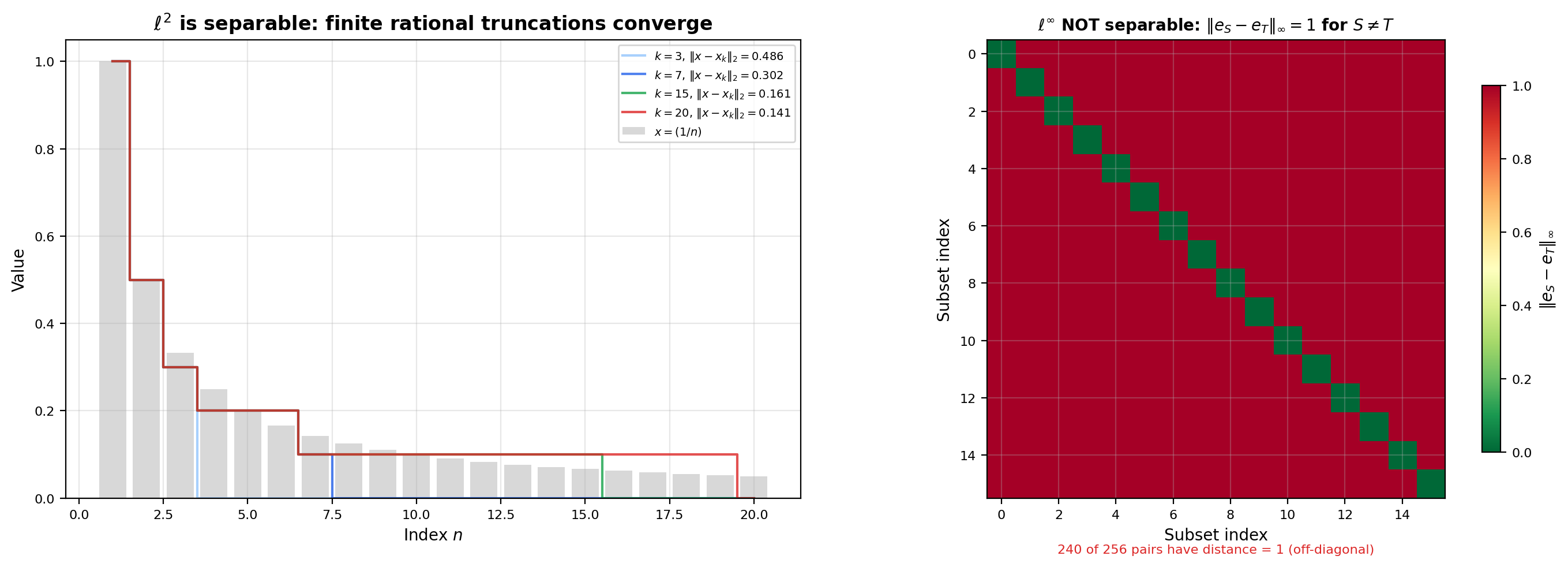
- for is separable.
- is NOT separable. Consider the uncountable family of sequences for . For , . Any dense subset must have a distinct element within distance of each , so it must be uncountable.
💡 Remark 8 (Separability and Computability)
In ML, we work with a finite number of data points and parameters. Separability ensures that the function space can be “reached” by finite approximations — countable dense subsets serve as computational proxies for the full space. Non-separable spaces like are pathological from a computational perspective: no countable algorithm can approximate all elements.
12. Connections to Statistics
Banach-space machinery underlies empirical-process theory and the operator-theoretic view of regression.
Empirical processes as Banach-valued
The empirical process lives in , the Banach space of bounded functions on with the sup norm. Donsker’s theorem is a Banach-valued CLT: converges in distribution (in ) to a Gaussian process indexed by . See formalStatistics Empirical Processes.
Regression as bounded linear projection
The OLS projection of onto is a bounded linear operator on (a finite-dimensional Banach/Hilbert space). The operator-theoretic view generalizes cleanly to infinite-dimensional regression problems — splines, Gaussian processes, and functional regression all sit on this Banach-space foundation. See formalStatistics Linear Regression.
13. Connections to ML
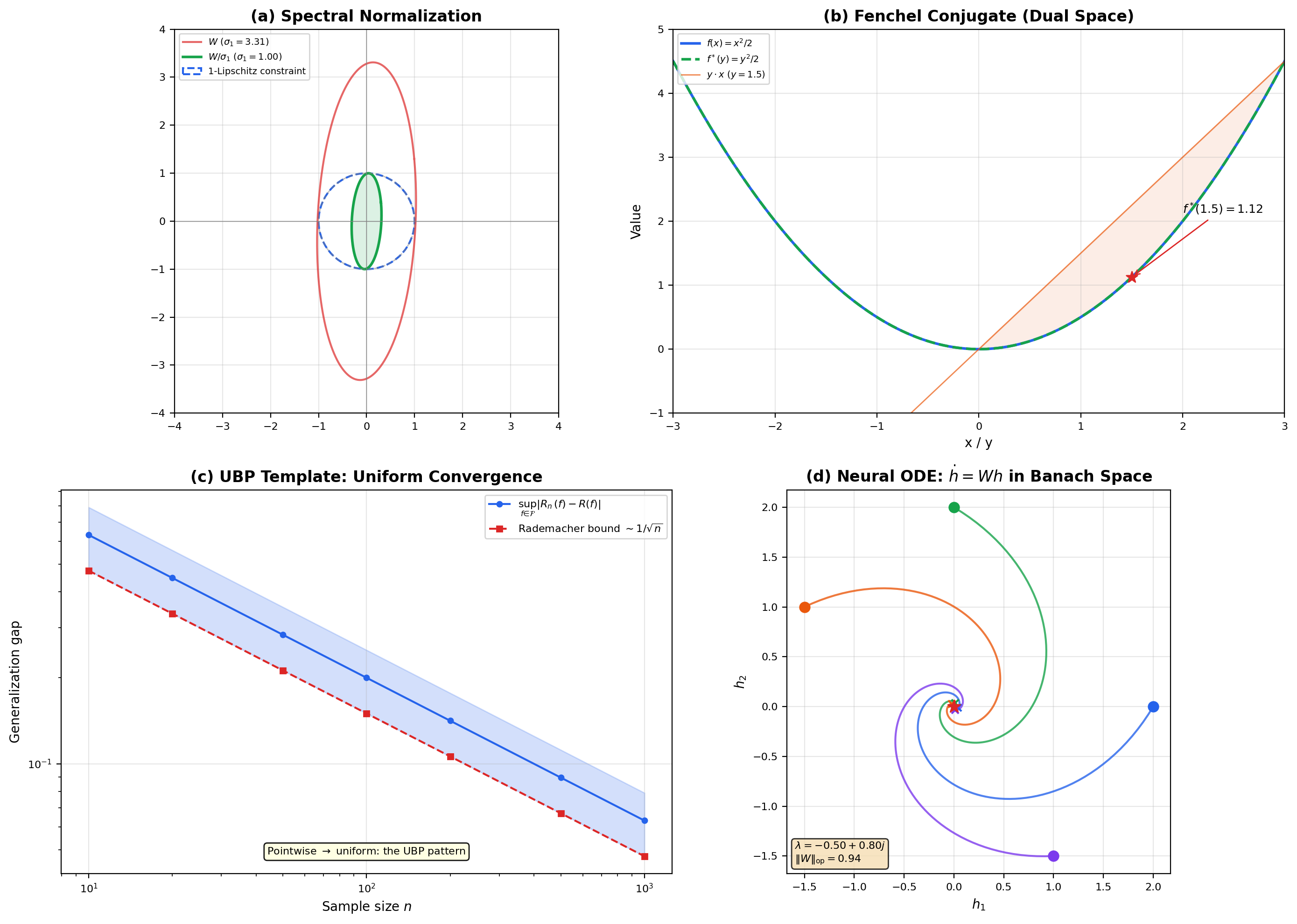
📝 Example 13 (Spectral Normalization and Operator Norms)
In Wasserstein GANs, the discriminator (critic) must be 1-Lipschitz: for all . For a linear layer , this means where is the largest singular value. Spectral normalization replaces with after each gradient step, enforcing the operator-norm constraint directly.
For deep networks with layers , the Lipschitz constant of the composition is at most — the operator norm composes multiplicatively. Controlling each layer’s operator norm controls the network’s global Lipschitz constant.
📝 Example 14 (Dual Spaces and Fenchel Conjugates)
The Fenchel conjugate (convex conjugate) of is:
where . This is fundamentally a dual-space operation: lives on , not on .
Mirror descent generalizes gradient descent from Hilbert spaces (where ) to Banach spaces: the update uses the Bregman divergence associated with a convex function , and the gradient maps between and . This is why online learning with the entropic regularizer (KL divergence) works on the probability simplex — the simplex lives in , and mirror descent uses the dual geometry.
📝 Example 15 (Uniform Boundedness and Generalization)
The empirical risk functional defines, for each data point , a bounded linear functional on the function space. Uniform convergence of to the population risk is a statement about the uniform boundedness of these evaluation functionals restricted to a hypothesis class .
The UBP’s message — “pointwise bounds imply uniform bounds for families of operators on Banach spaces” — is the functional-analytic template for Rademacher complexity bounds and VC-dimension arguments.
📝 Example 16 (Banach Spaces in Neural ODE Theory)
Neural ODEs model the hidden state evolution as where is a neural network. The solution operator is a bounded operator, and the theory of existence and uniqueness uses the Banach fixed-point theorem (Topic 29, Theorem 7) in the Banach space . Stability analysis requires operator-norm estimates on the Jacobian .
14. Computational Notes
Working Python implementations of the key computational ideas in this topic.
Computing operator norms. For a matrix :
- Spectral norm (ℓ² → ℓ²):
np.linalg.svd(A, compute_uv=False)[0]returns . - ℓ¹ → ℓ¹ norm:
np.abs(A).sum(axis=0).max()(maximum absolute column sum). - ℓ∞ → ℓ∞ norm:
np.abs(A).sum(axis=1).max()(maximum absolute row sum).
Spectral normalization (simplified power iteration):
# Estimate σ₁(W) via power iteration
u = np.random.randn(W.shape[0]); u /= np.linalg.norm(u)
for _ in range(10):
    v = W.T @ u; v /= np.linalg.norm(v)
    u = W @ v;   u /= np.linalg.norm(u)
sigma_1 = u @ W @ v
W_normalized = W / sigma_1
Fenchel conjugate for common cases:
- Quadratic: has .
- Entropic: on the simplex has (log-sum-exp).
15. Summary and Key Results
The dependency structure of this topic:
Foundation: Normed vector spaces (Definition 1) add algebraic structure to metric spaces. Every norm induces a translation-invariant, absolutely homogeneous metric. In finite dimensions, all norms are equivalent (Theorem 1); in infinite dimensions, they are not.
Completeness: Banach spaces (Definition 2) are complete normed spaces. Completeness is equivalent to absolute convergence implying convergence (Proposition 1). The operator space is Banach when is Banach (Theorem 2) — the dual space is always Banach.
The engine: The Baire Category Theorem (Theorem 3) — a complete metric space is not meager in itself — is the single result that powers the three pillars.
The three pillars:
- Uniform Boundedness Principle (Theorem 4): pointwise bounded uniformly bounded.
- Open Mapping Theorem (Theorem 5): surjective bounded linear operators are open.
- Closed Graph Theorem (Theorem 6): closed graph bounded.
Dual spaces: is the Banach space of bounded linear functionals (Definition 7). Hahn-Banach (Theorem 7) guarantees norm-preserving extensions. The canonical duality and connect to Topics 27–28.
16. Looking Ahead — From Banach to Hilbert
Every Hilbert space is a Banach space, but the converse fails — is Banach but not Hilbert (the parallelogram law fails). The passage from Banach to Hilbert is the addition of an inner product: a bilinear form that induces the norm via .
This additional structure buys three powerful tools that Banach spaces lack:
- Orthogonal projections — the closest point in a closed convex set. In Banach spaces, closest points may not exist or not be unique; in Hilbert spaces, the projection theorem guarantees both.
- The Riesz representation theorem — , every Hilbert space is self-dual. This is dramatically simpler than the Banach-space dual structure.
- RKHS foundations — reproducing kernels as inner-product evaluations, connecting Hilbert space theory to kernel methods in ML.
Connections & Further Reading
Prerequisites — topics you need first
Metric Spaces & Topology
Topic 29 established the metric space framework — completeness, compactness, and continuity in abstract spaces. Topic 30 adds algebraic structure (vector space + norm) and delivers the Baire Category Theorem and its three consequences, all deferred from Topic 29.
Lp Spaces
Topic 27 proved Lp spaces are complete normed spaces (Riesz-Fischer) and sketched the duality (Lp)* = Lq. Topic 30 provides the abstract Banach space theory that Lp spaces exemplify, and cites the duality result as the canonical dual-space computation.
Radon-Nikodym & Probability Densities
Topic 28 proved the Radon-Nikodym theorem, which Topic 27 used in the duality proof sketch. The (Lp)* = Lq isomorphism cited in Topic 30 depends on Radon-Nikodym.
Uniform Convergence
Topic 4 established C([a,b]) with the sup-norm as a natural function space. Topic 30 identifies C([a,b]) as a Banach space and uses it as a key example throughout.
Approximation Theory
Topic 20 used density of polynomials in C[a,b] under the sup-norm. Topic 30 formalizes best approximation in normed spaces and connects density to separability.
Completeness & Compactness
Topic 3 established completeness of R. The Baire Category Theorem in Topic 30 generalizes this: R is not a countable union of nowhere-dense sets, and neither is any complete metric space.
Where this leads — next in formalCalculus
Inner Product & Hilbert Spaces
Every Hilbert space is a Banach space with an extra inner-product structure. That extra structure unlocks orthogonal projections, the Riesz representation theorem (H* ≅ H, self-duality), and RKHS foundations — tools that Banach spaces alone cannot provide.
Calculus of Variations
Optimization of functionals on Banach and Sobolev spaces. The direct method exploits weak compactness and lower semicontinuity in reflexive spaces — the Banach-space machinery from this topic is the infrastructure variational problems run on.
On to formalStatistics — where this calculus powers inference
Empirical Processes
The empirical process X_n: 𝓕 → ℝ lives in ℓ^∞(𝓕), the Banach space of bounded functions on 𝓕 with the sup norm. Donsker's theorem is a Banach-valued CLT: √n(P_n - P) converges in distribution (in ℓ^∞(𝓕)) to a Gaussian process.
Linear Regression
The projection of y onto col(X) — the OLS fit — is a bounded linear operator on ℝⁿ (a finite-dimensional Banach/Hilbert space). The operator-theoretic view generalizes to infinite-dimensional regression problems.
On to formalML — where this calculus powers ML
Gradient Descent
Operator norms bound Lipschitz constants of gradient maps. The Open Mapping Theorem guarantees bounded inverses of surjective linear layers, controlling gradient flow through deep networks. Mirror descent operates in Banach spaces with Bregman divergences, and the dual-space geometry — Fenchel conjugates, subgradients in $X^*$ — extends gradient descent beyond Hilbert spaces.
PAC Learning
The Uniform Boundedness Principle is the functional-analytic backbone of uniform convergence. Generalization bounds in PAC learning require function-class boundedness — a UBP consequence.
References
- book Kreyszig (1978). Functional Analysis Chapters 2-4 (normed spaces, Banach spaces, fundamental theorems). Excellent pedagogy for the advanced reader.
- book Rudin (1976). Principles of Mathematical Analysis Chapter 5 (differentiation and the Baire category theorem in the real-analysis context).
- book Folland (1999). Real Analysis: Modern Techniques and Their Applications Chapter 5 (elements of functional analysis). Clean treatment of the three pillars.
- book Brezis (2011). Functional Analysis, Sobolev Spaces and Partial Differential Equations Chapters 1-2 (Hahn-Banach, uniform boundedness, open mapping). Modern presentation with applications.
- book Rudin (1987). Real and Complex Analysis Chapter 5 (examples of Banach spaces, Baire category). The canonical graduate reference.