Metric Spaces & Topology
Generalizing distance beyond Euclidean space — from metric axioms through completeness and compactness to the contraction mapping theorem and Arzelà–Ascoli, with applications to fixed-point iteration, embedding spaces, and metric learning.
Abstract. Every machine learning algorithm that computes a distance — every k-nearest-neighbor lookup, every gradient descent step, every embedding similarity score — is operating in a metric space. This topic generalizes the completeness and compactness theory from Topic 3 beyond Euclidean space to arbitrary metric spaces, where the notion of distance is axiomatized by three properties: positivity, symmetry, and the triangle inequality. The payoff is immediate. The Banach Contraction Mapping Theorem guarantees that any contraction on a complete metric space has a unique fixed point — this single result explains why Picard iteration solves ODEs, why Newton's method converges, why value iteration in reinforcement learning finds the optimal policy, and why many iterative algorithms in machine learning are guaranteed to converge. The Arzelà–Ascoli theorem characterizes compact subsets of function spaces and explains when a sequence of functions must have a uniformly convergent subsequence. Along the way, we develop the language of topology — open and closed sets, continuity via preimages, and the distinction between metric and general topological spaces — that will power the remaining three topics in this track.
1. Why Metric Spaces?
Every machine learning algorithm that computes a distance is quietly operating in a metric space. The Euclidean distance in is the obvious example — it is what -nearest neighbors uses, what gradient descent steps respect, and what the word “similarity” means for Word2Vec embeddings. But Euclidean distance is not the only game in town, and for several of the questions we are about to ask, it is not even the right tool.
Three motivating puzzles set the stage.
Puzzle 1: Comparing functions. Given two continuous functions , how do we measure how far apart they are? One natural answer is the sup-norm distance , which we saw already in Uniform Convergence — it is the metric that makes “convergence” mean “uniform convergence.” But there are other answers: the integral-based distance , the distance , and many more. Each is a legitimate metric, and each gives a different geometric character. The framework we develop in this topic will explain why.
Puzzle 2: When does iteration converge? Suppose is a map from some space to itself and we iterate: start with , set , , and so on. When does the sequence converge, and when it does, to what? We are going to prove a theorem — the Banach Contraction Mapping Theorem — that answers this completely for any map that “shrinks distances.” The same theorem is why Picard iteration solves ordinary differential equations, why Newton’s method converges in a neighborhood of a simple root, and why reinforcement-learning value iteration finds the optimal policy. A single abstract result unifies half a dozen concrete convergence arguments.
Puzzle 3: Which function families are “small” enough to extract a convergent subsequence? In Topic 3 we proved the Bolzano–Weierstrass theorem: every bounded sequence in has a convergent subsequence. In this is simply false — the sequence is bounded in the sup-norm (each ), yet no subsequence converges uniformly. We flagged this counterexample in Topic 3 and promised to explain it here. The explanation is that “bounded” is the wrong condition in infinite dimensions; the right one involves equicontinuity, and the theorem that packages it is Arzelà–Ascoli.
These three puzzles are really one question asked three ways: what structure does a space need for the usual analytic intuition to work? The answer — the metric space axioms — is small, geometric, and surprisingly powerful. By the end of this topic we will have generalized completeness, compactness, and continuity from to arbitrary metric spaces, and we will have proved the two theorems that turn this machinery into concrete convergence guarantees for machine learning algorithms.
2. Metric Space Axioms and Examples
The metric space abstraction compresses the idea of “distance” into three axioms. Everything we prove from here down follows from these three statements and nothing else — which is what gives the theory its reach.
📐 Definition 1 (Metric Space)
A metric space is a pair consisting of a set and a function called a metric (or distance function) satisfying:
- Positivity: if and only if , and for all .
- Symmetry: for all .
- Triangle inequality: for all .
The three axioms are exactly the properties the word “distance” should have. Positivity says distance is never negative and vanishes only at a single point. Symmetry says the distance from to does not depend on which one you started at. The triangle inequality says that going via an intermediate point is never a shortcut. If any of these fail, the machinery we are about to build breaks — which is why metric learning papers spend so much effort ensuring their learned “distances” actually satisfy these properties. Examples build intuition faster than axioms; here are four canonical ones.
📝 Example 1 (The ℓᵖ Metrics on Rⁿ)
For , the metric on is
For the formula degenerates and we use
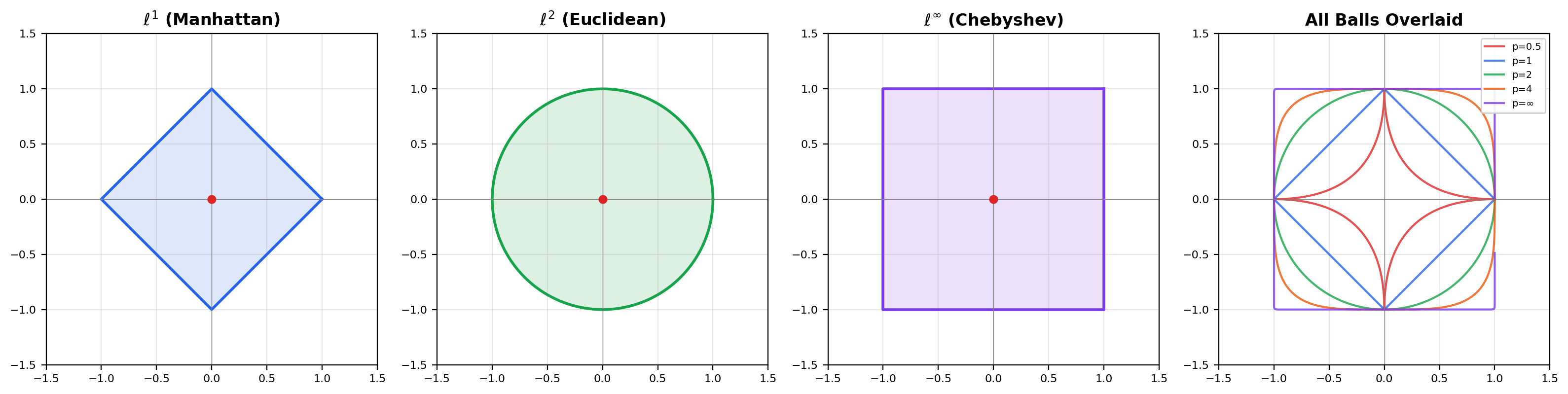
All three axioms are satisfied for every (the triangle inequality is Minkowski’s inequality). Three values of are worth remembering: gives the usual Euclidean distance, gives the “Manhattan” or taxicab distance, and gives the Chebyshev (max-coordinate) distance. In , the “unit ball” is a diamond for , a circle for , and a square for — the same set acquires three visibly different geometries depending on which metric we choose.
📝 Example 2 (The Sup-Norm Metric on C([a,b]))
The space of continuous real-valued functions on becomes a metric space under
Positivity and symmetry are immediate. The triangle inequality follows from the pointwise inequality by taking suprema on both sides. This is the same sup-norm that appeared in Uniform Convergence: a sequence converges to in this metric if and only if uniformly. Section 5 will prove that is complete — every Cauchy sequence converges — which is why the sup-norm is the right tool for function-space fixed-point arguments.
📝 Example 3 (The Discrete Metric)
On any set , define
All three axioms are trivial to verify. Under this metric every subset is open, every convergent sequence is eventually constant, and the “unit ball” contains only the single point . The discrete metric shows that metric-space theory applies to exotic settings — there is no requirement that look anything like — and it is a useful source of counterexamples whenever you suspect a theorem secretly needs continuity.
📝 Example 4 (Hamming Distance)
On the set of binary strings of length , the Hamming distance is
the number of coordinates in which and differ. Symmetry is clear, positivity is clear, and the triangle inequality holds because “coordinates where and differ” is a subset of “coordinates where and differ” “coordinates where and differ.” Hamming distance is the metric behind error-correcting codes and is directly relevant to discrete ML: training a classifier to produce outputs within Hamming distance of a target is a metric-space constraint.
💡 Remark 1 (Different Metrics, Different Topologies)
The same underlying set can carry many different metrics, and the choice shapes everything else: which sequences converge, which sets are open, which functions are continuous. In the , , and metrics all generate the same notion of “open set” (they are topologically equivalent — we will define this precisely in Section 8), so they all agree on which sequences converge. But the Hamming metric on is qualitatively different from the Euclidean metric on the same set viewed as a subset of : under Hamming distance, consecutive binary strings (differing in a single bit) are always at distance 1, but under Euclidean distance their positions depend on which bit changed. The metric determines the geometry, and the geometry determines the analysis.
3. Open Sets, Closed Sets, and the Language of Topology
With the metric in hand we can start building the vocabulary of topology: balls, open sets, closed sets, interiors, closures, boundaries. This is the language that every subsequent theorem in the topic will speak, and it is the same vocabulary Topic 3 used for — only now it works in any metric space.
📐 Definition 2 (Open and Closed Balls)
Let be a metric space, let , and let . The open ball of radius centered at is
The closed ball of radius centered at is
The open ball has a strict inequality; the closed ball includes the boundary sphere. In with these are the familiar solid balls without and with their bounding spheres. In with the sup-norm, the open ball is the set of all continuous functions whose graph lies strictly within an -tube around the graph of — exactly the “uniform tube” that Topic 4 used to define uniform convergence.
📐 Definition 3 (Open and Closed Sets)
A set is open if for every point there exists some such that the open ball is entirely contained in :
A set is closed if its complement is open.
A set is open if every point has some breathing room: a small open ball around it that stays inside the set. A set is closed if its complement has that property. Note that “closed” does not mean “not open” — the empty set and the whole space are both open and closed in every metric space (check the definitions directly), and in the discrete metric every subset is both open and closed. Openness and closedness are more subtle than they look.
🔷 Proposition 1 (Properties of Open and Closed Sets)
In any metric space :
- and are both open and closed.
- Arbitrary unions of open sets are open.
- Finite intersections of open sets are open.
- Arbitrary intersections of closed sets are closed.
- Finite unions of closed sets are closed.
The asymmetry between “arbitrary” and “finite” matters. Arbitrary intersections of open sets need not be open — the classic example is , an intersection of open intervals whose limit is a single point, which is not open. Similarly, arbitrary unions of closed sets need not be closed. The finiteness restriction in items 3 and 5 is therefore essential, not cosmetic.
📐 Definition 4 (Interior, Closure, Boundary, Limit Point)
For a subset :
- The interior is the union of all open sets contained in ; equivalently, it is the largest open set inside .
- The closure is the intersection of all closed sets containing ; equivalently, it is the smallest closed set that contains .
- The boundary is .
- A point is a limit point of if every open ball contains a point of other than .
Two facts follow immediately. First, : the interior is contained in , which is contained in the closure. Second, is open exactly when , and is closed exactly when — these are not additional hypotheses but equivalent characterizations. The closure can also be described as , which is often the easiest way to compute it in practice.
📝 Example 5 (Open Sets in C([0,1]))
In with the sup-norm, the open ball consists of all continuous functions whose graph lies within the horizontal band . A set is open precisely when for every we can find a small enough so that every continuous function inside the -tube around is also in . This is exactly the “-tube” picture from Topic 4’s visualization of uniform convergence — the only difference is that now we are thinking of a tube as an open ball in a metric space.
![Four-panel figure: interior, closure, and boundary of a subset of R; an open ball in R²; an ε-tube open ball in C([0,1]); and the trivial "balls" of the discrete metric.](/images/topics/metric-spaces/open-closed-sets.png)
4. Continuity in Metric Spaces
Continuity is the next concept that lifts from to arbitrary metric spaces. We give three equivalent characterizations — an - definition, a sequential definition, and a preimage-of-open-set definition — and show that all three are equivalent. The third characterization is the conceptual payoff: it describes continuity using only the structure of open sets, which is what lets the definition generalize to spaces without a metric at all.
📐 Definition 5 (Continuity (ε–δ))
Let and be metric spaces. A function is continuous at a point if for every there exists such that
The function is continuous (on all of ) if it is continuous at every point of .
This is the same - definition we used in Topic 2 for real-valued functions of a real variable, with and replacing the absolute value. Now the three characterizations.
🔷 Theorem 1 (Three Characterizations of Continuity)
Let be a function between metric spaces. The following are equivalent:
- is continuous at every point of (the – definition).
- For every convergent sequence in , we have in .
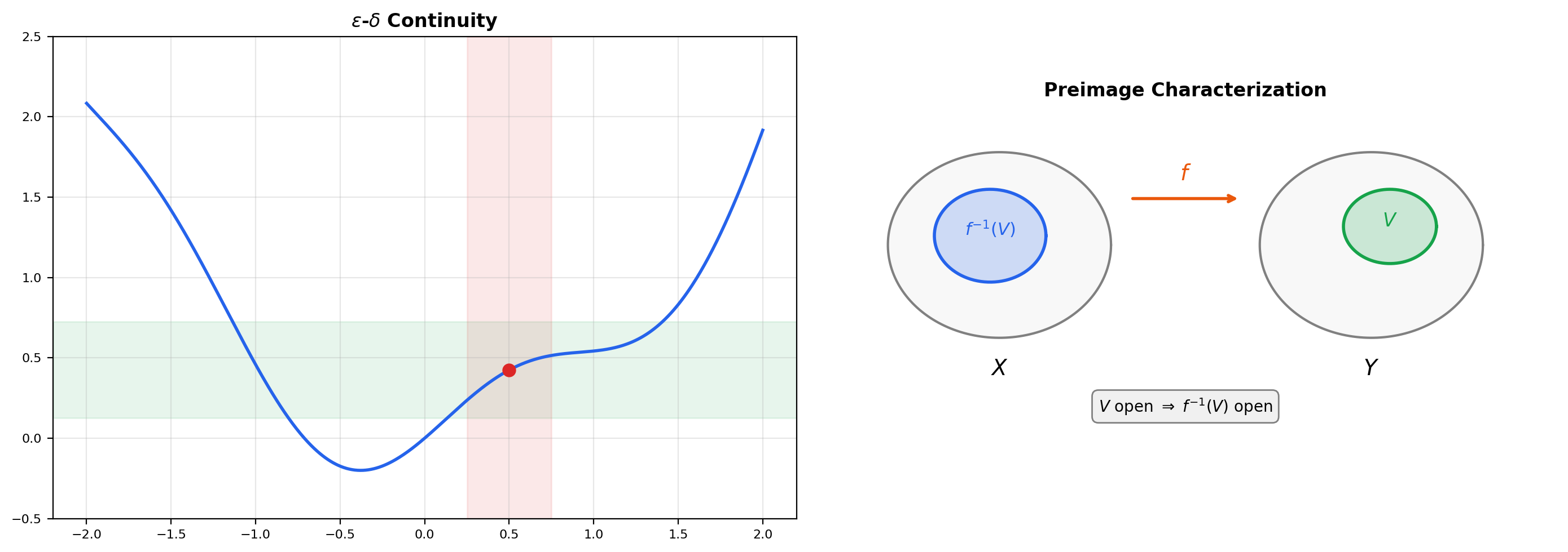
- For every open set , the preimage is open in .
Proof.
We prove the three implications .
. Assume is continuous at every point, let in , and fix . Continuity at gives some such that implies . Since , there exists such that for all we have , and therefore . This is exactly the statement that .
. Assume sequential continuity, let be open, and let . We need to show some ball is contained in . Suppose not. Then for every there exists a point with but . By construction , so by sequential continuity . But and is open, so some ball is contained in , which means for all sufficiently large — contradicting .
. Assume preimages of open sets are open, let , and fix . The open ball is open in , so by hypothesis its preimage is open in and contains . By the definition of “open” we can find some with , which rewrites as: . That is the – condition at . Since was arbitrary, is continuous.
💡 Remark 2 (Why Preimages Matter)
Characterization (3) is the conceptual leap: it describes continuity entirely in terms of the structure of open sets, with no reference to distances or sequences. This is what lets the definition generalize to topological spaces in Section 8, where there may be no metric at all. In metric spaces all three characterizations are equivalent — we just proved it — so the preimage formulation looks like one more way to say the same thing. The power of (3) only becomes apparent when we leave metrics behind: in an arbitrary topological space, the – definition is not even expressible, and the sequential definition can fail in strange ways. The preimage characterization is the universally correct one.
📐 Definition 6 (Lipschitz Continuity)
A function is Lipschitz continuous with constant if
The smallest such is called the Lipschitz constant of . If the map is called a contraction, and this case will drive Section 7.
Lipschitz continuity is strictly stronger than continuity (every Lipschitz function is continuous, take ) and strictly weaker than differentiability with bounded derivative (every such function is Lipschitz on a bounded domain). For ML purposes, Lipschitz constants quantify how rapidly a function can change: they control the convergence rate of gradient descent, the sensitivity of a neural network to input perturbations, and the stability of numerical ODE solvers. We will see concrete examples in Sections 7 and 10.
5. Completeness in Metric Spaces
Completeness generalizes the Cauchy-completeness of (Topic 3, Section 1) to arbitrary metric spaces. The crucial new example — the one that powers every fixed-point argument in the rest of the topic — is that with the sup-norm is complete.
📐 Definition 7 (Cauchy Sequence in a Metric Space)
A sequence in a metric space is Cauchy if for every there exists such that
📐 Definition 8 (Complete Metric Space)
A metric space is complete if every Cauchy sequence in converges to a limit that is also in .
Cauchy says the terms of the sequence eventually cluster together; complete says that clustering is enough to guarantee a limit. The two concepts are linked but distinct: is not complete (the sequence of decimal approximations to is Cauchy in but has no rational limit), while is complete — and this is exactly how was constructed from (by filling in the missing limits).
📝 Example 6 (Completeness of Rⁿ)
is complete by the Cauchy-completeness theorem from Topic 3, Section 1. is complete under any of the metrics: if is a Cauchy sequence in , then each coordinate sequence is Cauchy in (because ), so each coordinate converges to some limit , and coordinate-wise convergence in implies convergence. This is the same argument Topic 3 ran for the Euclidean metric; all it needed was the coordinate inequality, which holds for every .
🔷 Theorem 2 (Completeness of C([a,b]))
The space with the sup-norm metric is complete.
Proof.
Let be a Cauchy sequence in . We need to exhibit a continuous function such that .
Step 1: Pointwise limit exists. For each , the sequence of real numbers is Cauchy in , because
Since is complete, converges to some real number, which we define to be . This gives a function as the pointwise limit.
Step 2: Convergence is uniform. Given , the Cauchy condition gives such that for all . Fix and any . Letting in the inequality , the right side stays and the left side converges to . Therefore for all , which means . Since was arbitrary, uniformly.
Step 3: The limit is continuous. This is exactly the Uniform Limit Theorem from Uniform Convergence: a uniform limit of continuous functions is continuous. So , and the previous step says . The sequence converges in the sup-norm metric, as needed.
This theorem is small but it is the backbone of the rest of the topic. Every fixed-point argument in Sections 7 and 10 — Picard iteration, Newton’s method, Bellman iteration — lives inside or an analogous function space, and every such argument needs to know that Cauchy sequences converge. The completeness of is what lets us “extract a limit” at the end of each proof.
📝 Example 7 (Incompleteness of C([0,1]) under a Different Metric)
The same set is not complete under the integral-based metric
Consider the sequence of continuous functions on defined to be on , linear from to on , and on — a “ramp” of width around . For large , the difference is supported in a shrinking interval of length , so as : the sequence is Cauchy in . But its pointwise limit is the step function that jumps from to at , which is discontinuous — and no continuous function can be the -limit of this Cauchy sequence. So is not complete. The completeness of a space depends on the metric, not just the set.
💡 Remark 3 (The Completion Theorem)
Every metric space has a completion: a complete metric space together with an isometric embedding such that is dense in . The construction mirrors how is built from : form equivalence classes of Cauchy sequences in , where two Cauchy sequences are equivalent if their interleaving is also Cauchy. The completion of is a larger space containing limits like our ramp-sequence step function — a space that analysts call and that shows up constantly in modern machine learning. We state the completion theorem as a fact rather than proving it in detail; Munkres, Chapter 3, has the full construction.
![Three-panel figure: a Cauchy sequence in R converging; a Cauchy sequence in (C([0,1]), sup-norm) converging uniformly; the ramp-sequence Cauchy in d₂ but with no continuous limit.](/images/topics/metric-spaces/completeness-cauchy.png)
6. Compactness in Metric Spaces
Compactness is the most technically important concept in the topic. In , the Heine–Borel theorem from Topic 3 told us that compact sets are exactly the closed and bounded ones. In general metric spaces this is false — and the proof of “why it fails” is the counterexample we promised back in Topic 3. In this section we give the general definition, prove the three-way equivalence with sequential compactness and total boundedness, and visualize the counterexample.
📐 Definition 9 (Open-Cover Compactness)
A metric space is compact if every open cover of has a finite subcover: whenever with each open, there is a finite set such that . A subset is compact if it is compact as a metric space under the restricted metric.
📐 Definition 10 (Sequential Compactness)
A metric space is sequentially compact if every sequence in has a convergent subsequence.
📐 Definition 11 (Total Boundedness)
A metric space is totally bounded if for every there exist finitely many points such that the corresponding -balls cover :
The collection is called a finite -net for .
Total boundedness is strictly stronger than boundedness. A bounded set of a metric space only needs to fit inside a single large ball; a totally bounded set needs to be approximable, at every resolution , by a finite number of points. In the two concepts agree (because is finite-dimensional and a single bounded ball contains only “finitely many balls-worth of material”). In infinite-dimensional spaces they come apart dramatically — and that is exactly why Heine–Borel fails in .
🔷 Theorem 3 (Compactness Equivalence in Metric Spaces)
For a metric space , the following three conditions are equivalent:
- is compact (every open cover has a finite subcover).
- is sequentially compact (every sequence has a convergent subsequence).
- is complete and totally bounded.
Proof.
We sketch the three directions. Full proofs are in Munkres, Chapter 3, or Rudin, Chapter 2.
. Suppose is compact and let be a sequence with no convergent subsequence. Then no point is a cluster point of , so each has an open ball containing only finitely many terms of the sequence. These balls form an open cover of . Compactness gives a finite subcover, which therefore contains only finitely many terms in total — but the full sequence has infinitely many terms, a contradiction.
. Sequential compactness implies completeness: a Cauchy sequence has a convergent subsequence by hypothesis, and a Cauchy sequence with a convergent subsequence converges to the same limit (standard Cauchy-subsequence lemma). For total boundedness, suppose has no finite -net for some . Pick any . Since is not all of , pick . Since is not all of , pick outside both balls. Continuing, we construct a sequence with pairwise distances , which has no convergent subsequence — contradicting sequential compactness.
(the hardest direction). Suppose is complete and totally bounded but has an open cover with no finite subcover. Total boundedness gives a finite -net; at least one of the balls intersected with has no finite subcover (otherwise combining them would give a finite subcover of the whole space). Pick one such ball, shrink to , and apply total boundedness inside that ball to get a smaller uncovered ball . Iterating, we obtain a nested sequence of sets with diameters shrinking to zero; picking one point from each gives a Cauchy sequence. By completeness it converges to some limit , which belongs to some in the cover. Because is open, contains a ball around , so covers all the tail sets in our nested sequence once they are small enough — giving a finite subcover for that tail after all, contradicting our construction.
💡 Remark 4 (Heine–Borel as a Special Case)
In , the Heine–Borel theorem from Completeness & Compactness in Rⁿ says compact ⟺ closed and bounded. This is a special case of the general three-way equivalence we just proved: in , bounded and totally bounded are the same thing (because is finite-dimensional, so a single bounded ball contains only finitely many small balls’ worth of volume). And a closed subset of a complete space is complete. So in , closed + bounded is the same as complete + totally bounded, which by Theorem 3 is the same as compact. The equivalence “bounded ⟺ totally bounded” fails in infinite dimensions — and we are about to see exactly how badly.
📝 Example 8 (The C([0,1]) Counterexample)
The closed unit ball in the sup-norm is closed and bounded, but not compact. This is the counterexample promised in Topic 3.
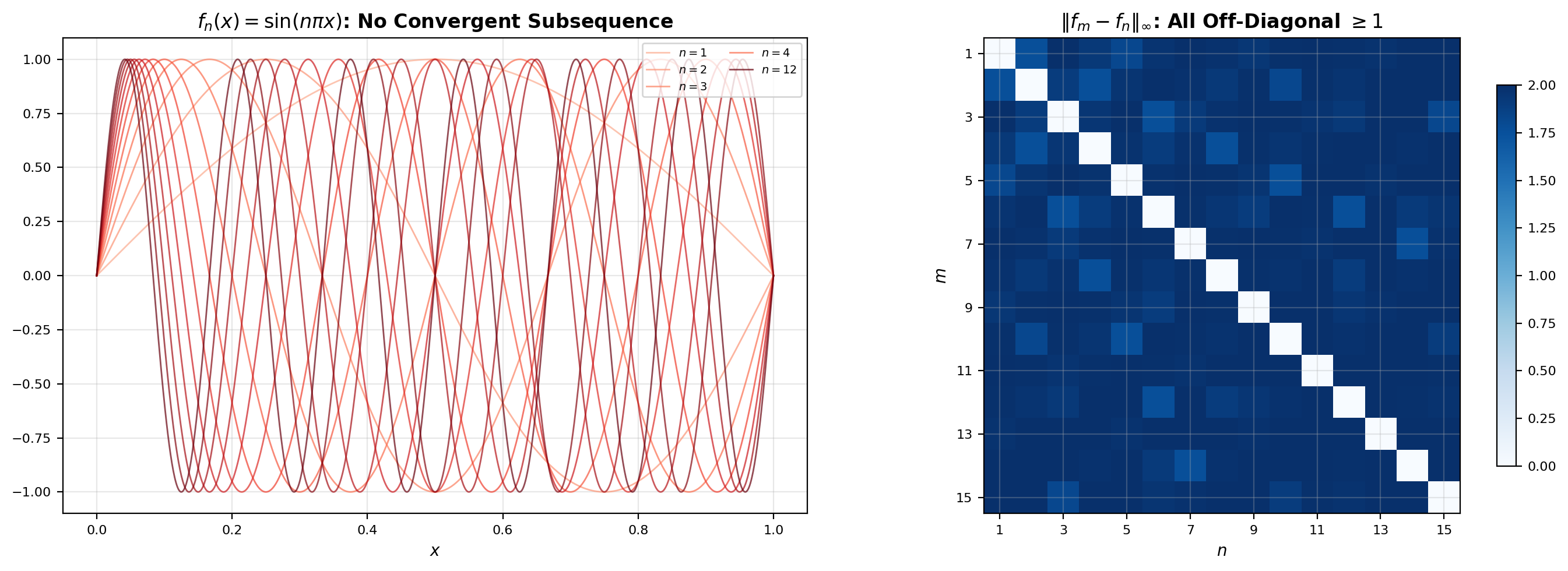
Proof. Consider the sequence for . Each is continuous and , so every . We claim that no subsequence of is Cauchy in the sup-norm — and therefore no subsequence converges, so is not sequentially compact and (by Theorem 3) not compact.
To see why, fix distinct indices . The functions and are orthogonal in :
Expanding using orthogonality and :
Now use the bound on : if the sup-norm of the difference were less than 1, the integral above would be less than 1. But the integral equals 1, so
Every pair of terms in the sequence is at sup-norm distance at least 1 — so no subsequence is Cauchy, and no subsequence converges.
The lesson. In an infinite-dimensional space, closed and bounded is not enough for compactness. The missing ingredient is equicontinuity: the family is bounded, but the functions “wiggle faster and faster” — for large there is no single that controls uniformly across the family. We will name this obstruction and package it into the Arzelà–Ascoli theorem in Section 9.
7. The Contraction Mapping Theorem
We now prove the theorem that justifies most of the fixed-point arguments scattered throughout the rest of this curriculum. It is short, clean, and extraordinarily useful: four earlier topics have been waiting to cite it.
🔷 Theorem 4 (Banach Contraction Mapping Theorem)
Let be a complete metric space and let be a contraction with Lipschitz constant , meaning
Then:
- has a unique fixed point — a point with .
- For any starting point , the iterates converge to .
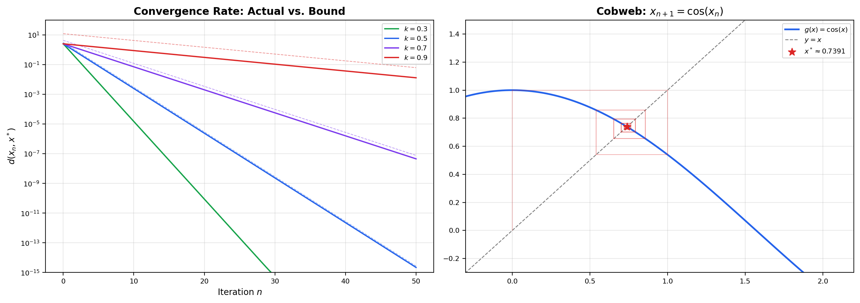
- The convergence rate is geometric: .
Proof.
Fix a starting point and define the iterates . The contraction property applied to consecutive iterates gives
By induction, this bound extends to
Now we show is Cauchy. For any , the triangle inequality stacks up consecutive-iterate bounds:
The geometric-series tail bound gives , so
Since , the right-hand side tends to as uniformly in — the sequence is Cauchy. Because is complete, converges to some limit .
Next we show is a fixed point. Contractions are Lipschitz (with constant ), hence continuous, so we can pass through the limit:
Uniqueness: suppose is another fixed point of . Then
Since , this forces , so .
Finally, the convergence rate. Letting in the Cauchy-tail bound , the left side converges to , proving
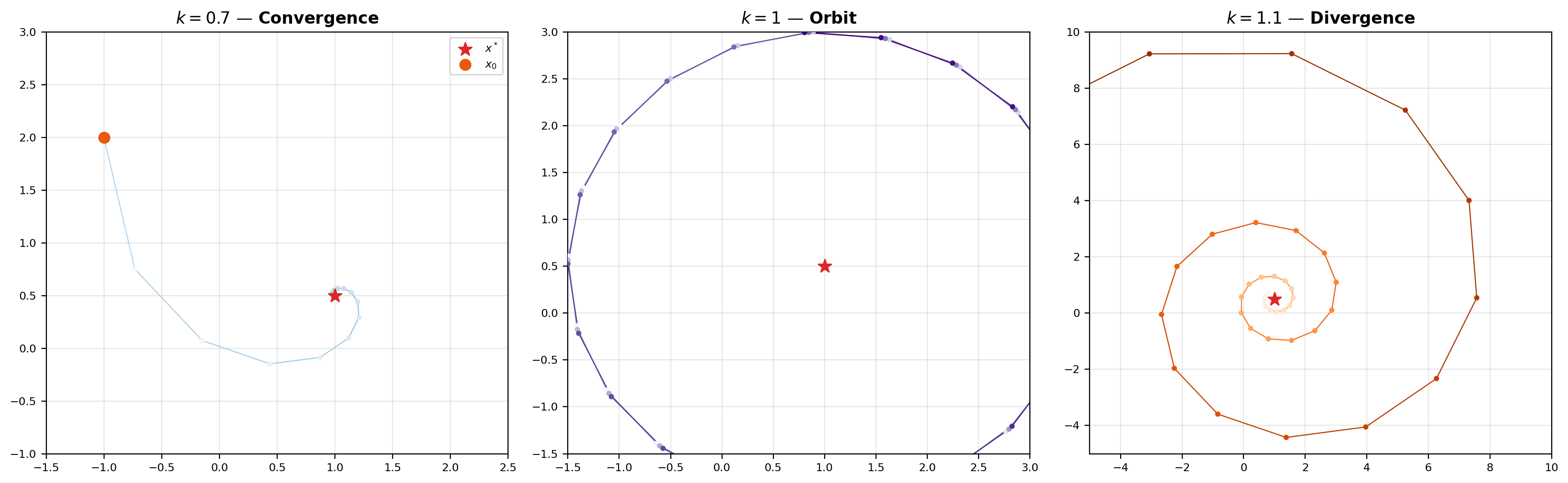
Three things to note. First, the theorem tells us nothing about which starting point to use — any works, and they all converge to the same fixed point. Second, the rate bound is sharp enough to give a stopping criterion: after iterations, the distance to is at most times the first step , a quantity we can measure after one evaluation of . Third, the contraction hypothesis is strict: at the theorem breaks, as the viz below demonstrates by letting you set and watch iterates orbit instead of converging.
An affine map T(x) = k·Rθ·x + c with θ = 30°. Operator norm of k·Rθ is exactly k. Click anywhere in the plot to set a new starting point x₀; drag the slider to change k.
📝 Example 9 (Picard Iteration for ODEs)
The Picard–Lindelöf existence-and-uniqueness theorem for first-order ODEs from First-Order ODEs rewrites the initial-value problem , as the fixed-point equation
Defining the Picard operator , a fixed point of is exactly a solution of the ODE. Topic 21 showed that when is Lipschitz in its second argument with constant and we work on a short interval with , the Picard operator is a contraction on with the sup-norm — constant — and is complete by Theorem 2. The Banach theorem then produces a unique fixed point, which is the ODE solution. The abstract theorem we just proved is what makes Topic 21’s concrete argument go through.
📝 Example 10 (Newton Iteration for Implicit Methods)
The implicit Euler method from Numerical Methods for ODEs requires solving the nonlinear equation at each time step. Newton’s method reduces this to iterating . For sufficiently small , the derivative of at the root is bounded in norm by some , so by the mean value theorem is a contraction on a small neighborhood of the root and Banach’s theorem guarantees convergence. Topic 24 invoked this conclusion in its convergence analysis without proof; we have now proved the general result.
📝 Example 11 (The Inverse Function Theorem)
The proof of the Inverse Function Theorem in Topic 12 constructs a local inverse by setting up the fixed-point equation where is a map on a small ball in whose Jacobian is bounded below 1 in operator norm. Banach’s theorem then gives a unique fixed point, which is the preimage of the target point. The whole construction is a single application of Theorem 4 to a carefully chosen contraction — the argument was specialized to in Topic 12, but the contraction-mapping framework developed here shows why it works in full generality.
💡 Remark 5 (Bernstein Operators Are Not Contractions)
Topic 20 proved that Bernstein operators converge uniformly to on — a statement that lives entirely in the metric space . But is not a contraction: it does not uniformly shrink sup-norm distances between arbitrary functions. Bernstein convergence is therefore not an application of Theorem 4; it is a different kind of approximation phenomenon that happens to share the same ambient metric space. The general lesson: sitting inside a complete metric space does not automatically make every self-map a contraction, and density-of-polynomials results require separate machinery (probabilistic moment arguments in the Bernstein case). What Topic 20 does share with this topic is the underlying metric-space structure — the sup-norm distance between and is how “convergence” is defined there, and that distance is a metric in exactly the sense defined here.
8. General Topology — Beyond Metric Spaces
Everything we have done so far has used the metric . But many of the concepts — continuity, open sets, closure, compactness — make sense in spaces where there is no metric at all, provided you know which sets are “open.” This section introduces the general notion of a topological space and explains why the preimage characterization of continuity is the one that generalizes.
📐 Definition 12 (Topological Space)
A topological space is a pair where is a set and is a collection of subsets of — called open sets — satisfying:
- and .
- Arbitrary unions of elements of are in .
- Finite intersections of elements of are in .
The collection is called a topology on . A metric space induces a topology by Proposition 1, so every metric space is a topological space. But there are topological spaces with no compatible metric, and those are strictly more general.
The three axioms are exactly the properties Proposition 1 established for metric-space open sets. Any collection of subsets satisfying them qualifies as a topology, regardless of whether it came from a metric. The question is whether all topologies come from metrics — and the answer is no.
📝 Example 12 (The Cofinite Topology)
Let be an uncountable set — for concreteness, take . Define to consist of the empty set together with all subsets whose complement is finite:
This is a topology: the empty set and are in , arbitrary unions of cofinite sets are cofinite (their complement is an intersection of finite sets, which is finite), and finite intersections of cofinite sets are cofinite (their complement is a finite union of finite sets, which is finite). So is a valid topological space.
But is not metrizable: there is no metric that generates this topology. Here is one quick reason. In the cofinite topology, any two non-empty open sets must intersect (the union of their complements is finite, so the intersection of the sets themselves is cofinite, hence non-empty). So for any two distinct points , every neighborhood of intersects every neighborhood of . In a metric space we can always separate distinct points by disjoint balls and — a property called the Hausdorff property. The cofinite topology on an uncountable set fails this, so no metric can generate it.
📐 Definition 13 (Continuity in Topological Spaces)
A function between topological spaces is continuous if for every open set , the preimage .
This is characterization (3) from Theorem 1 — the preimage-of-open-set condition — lifted verbatim to the topological setting. It is the only definition that works universally: the - definition requires a metric, and the sequential definition fails in non-first-countable spaces (where there are “too many” open sets for sequences to detect). In metric spaces all three definitions coincide, as we proved in Theorem 1; in general topology, we start with (3) and take the other two only when the space is metrizable.
📐 Definition 14 (Homeomorphism)
A homeomorphism between topological spaces and is a bijection such that both and are continuous. Two spaces related by a homeomorphism are topologically equivalent — they have the same open sets up to relabeling, the same convergence, the same compactness properties, and the same connectedness properties.
Homeomorphism is the “sameness” relation for topological spaces. Two very different-looking metric spaces can be topologically equivalent — for example, the open interval and the whole real line are homeomorphic (via any monotone continuous bijection like ), even though one has finite diameter and the other doesn’t. The metric “forgot” when we reduced to the topology.
💡 Remark 6 (Metrization and Fundamental Groups)
Topic 15 mentioned simply connected domains and fundamental groups as the setting for its discussion of conservative vector fields and path independence. These concepts live at the general-topology level: a domain is simply connected if every closed loop in it can be continuously contracted to a point, a property defined entirely in terms of continuous maps (homotopies of loops), and the fundamental group classifies loops up to continuous deformation. Fundamental groups make sense in any topological space and are preserved by homeomorphism — they are a topological invariant. Metric spaces inherit these invariants whenever they carry the metric-induced topology, which is almost always in analysis. The Urysohn Metrization Theorem gives a clean sufficient condition: a topological space is metrizable if (and essentially only if) it is second-countable, regular, and Hausdorff. Most spaces that appear in analysis satisfy these conditions, which is why metric-space theory covers so much ground. But the topological vocabulary — connectedness, path-connectedness, fundamental groups, homotopy — belongs to the general theory, not to metric spaces in particular.
9. Equicontinuity and the Arzelà–Ascoli Theorem
In Section 6 we saw that the closed unit ball of is not compact — the sequence has no convergent subsequence. The Arzelà–Ascoli theorem identifies exactly what extra condition is needed to restore compactness in function spaces: equicontinuity. Topic 4 introduced the concept and promised the proof; we pay that debt now.
📐 Definition 15 (Equicontinuity)
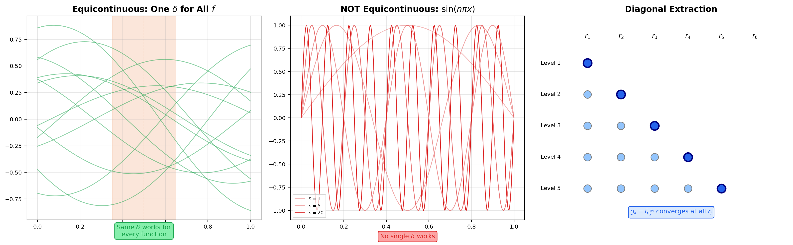
A family is equicontinuous if for every there exists a single — depending on but not on — such that for every and every with :
This is the concept Topic 4 introduced in the context of equicontinuity figures. The crucial word is single: uniform continuity of a single function says there is one that works for all points at once; equicontinuity of a family says there is one that works for all points and all functions at once. The family fails equicontinuity because faster-wiggling functions need smaller ‘s — no single choice works for the whole family. By contrast, any family of functions with a uniform Lipschitz bound (say for all in the family) is automatically equicontinuous: take .
📐 Definition 16 (Uniform Boundedness of a Family)
A family is uniformly bounded if there exists such that
Equivalently, the family fits inside a single closed ball of the sup-norm: for all .
🔷 Theorem 5 (Arzelà–Ascoli)
A subset (with the sup-norm metric) has compact closure if and only if is uniformly bounded and equicontinuous.
Equivalently: every uniformly bounded and equicontinuous sequence in has a subsequence that converges uniformly.
Proof.
We prove both directions. The forward direction is the routine one; the reverse direction is the workhorse “diagonal subsequence” argument.
() Uniformly bounded + equicontinuous ⟹ sequentially compact closure. Let be a sequence in . We will extract a subsequence that is Cauchy in the sup-norm; by completeness of (Theorem 2) it then converges, proving sequential compactness.
Step 1: pointwise convergence on a countable dense set. Enumerate the rationals in as — a countable dense set. At , the sequence of real numbers is bounded (by uniform boundedness of ), so by the Bolzano-Weierstrass theorem it has a convergent subsequence, which we index as . Next, the sequence is bounded in , so we extract a further subsequence converging at — and still converging at , since subsequences of convergent sequences converge to the same limit. Iterate this procedure: at step we have a subsequence that converges at each of .
Step 2: diagonal subsequence. Define the diagonal subsequence . For every fixed rational , the sequence is a subsequence of , which converges at ; therefore converges too. So converges pointwise at every rational in .
Step 3: equicontinuity promotes pointwise to uniform. Given , equicontinuity gives such that
Cover by finitely many open intervals of length less than centered at rationals (we can pick rationals because they are dense). By Step 2, converges for each , so there exists such that for all and all :
Now let be arbitrary. Pick with . The triangle inequality gives
The first and third terms are each less than by equicontinuity (applied to and , which lie in ). The middle term is less than by the choice of . So for every , which means for all . The subsequence is Cauchy in , and by completeness it converges to some continuous function — which is the uniformly convergent subsequence we wanted.
() Compact closure ⟹ uniformly bounded + equicontinuous. Suppose is compact. Then it is bounded (compact sets are bounded in any metric space), so is uniformly bounded. For equicontinuity, fix . Compactness of in the sup-norm means we can cover it by finitely many sup-norm balls centered at functions . Each is continuous on the compact interval , hence uniformly continuous, giving some that makes whenever . Take .
Now for any , pick with . For :
Each of the three terms is bounded by , so . This bound holds for every with the same — equicontinuity.
📝 Example 13 (Why sin(nπx) Fails Arzelà–Ascoli)
The counterexample family from Section 6 is uniformly bounded ( for every ) but not equicontinuous. To see why, pick and ask for a that forces whenever . For any proposed , take large enough that , and take , . Then but
So the chosen fails at . No single works for the whole family — equicontinuity fails exactly because the functions oscillate faster and faster as grows. The failure of equicontinuity is precisely what blocks the Arzelà–Ascoli conclusion and explains why no subsequence converges.
💡 Remark 7 (Arzelà–Ascoli in Practice)
The theorem is the workhorse compactness criterion for function spaces. It gets used constantly in the existence theory for partial differential equations (bound the approximate solutions in a uniform-Lipschitz sense, extract a convergent subsequence, pass to the limit), in the regularity theory of calculus-of-variations minimizers, and in proving convergence of numerical schemes. In machine learning, it appears implicitly whenever you control the Lipschitz constant of a hypothesis class: a uniformly bounded, uniformly Lipschitz family of functions has compact closure in , which means you can always extract convergent subsequences from training trajectories and study their limits. Spectral norm regularization of neural networks is partially motivated by exactly this kind of Arzelà–Ascoli argument.
Click on the graph to probe equicontinuity at a point. Blue curves = extracted subsequence. Dashed red = limit approximation.
10. ML Connections — Distance, Fixed Points, and Embeddings
Everything in this topic has concrete machine learning payoffs. The Banach theorem explains why iterative algorithms converge; the metric-space axioms explain what “distance” must satisfy for similarity-based methods to work; the Arzelà–Ascoli theorem controls the compactness of function classes. Here are four connections that appear across modern ML.
📝 Example 14 (The Bellman Operator Is a Contraction)
In reinforcement learning, the Bellman optimality operator acts on bounded value functions by
where is the discount factor. Under the sup-norm , the space of bounded value functions on a finite state space is complete, and is a contraction with constant :
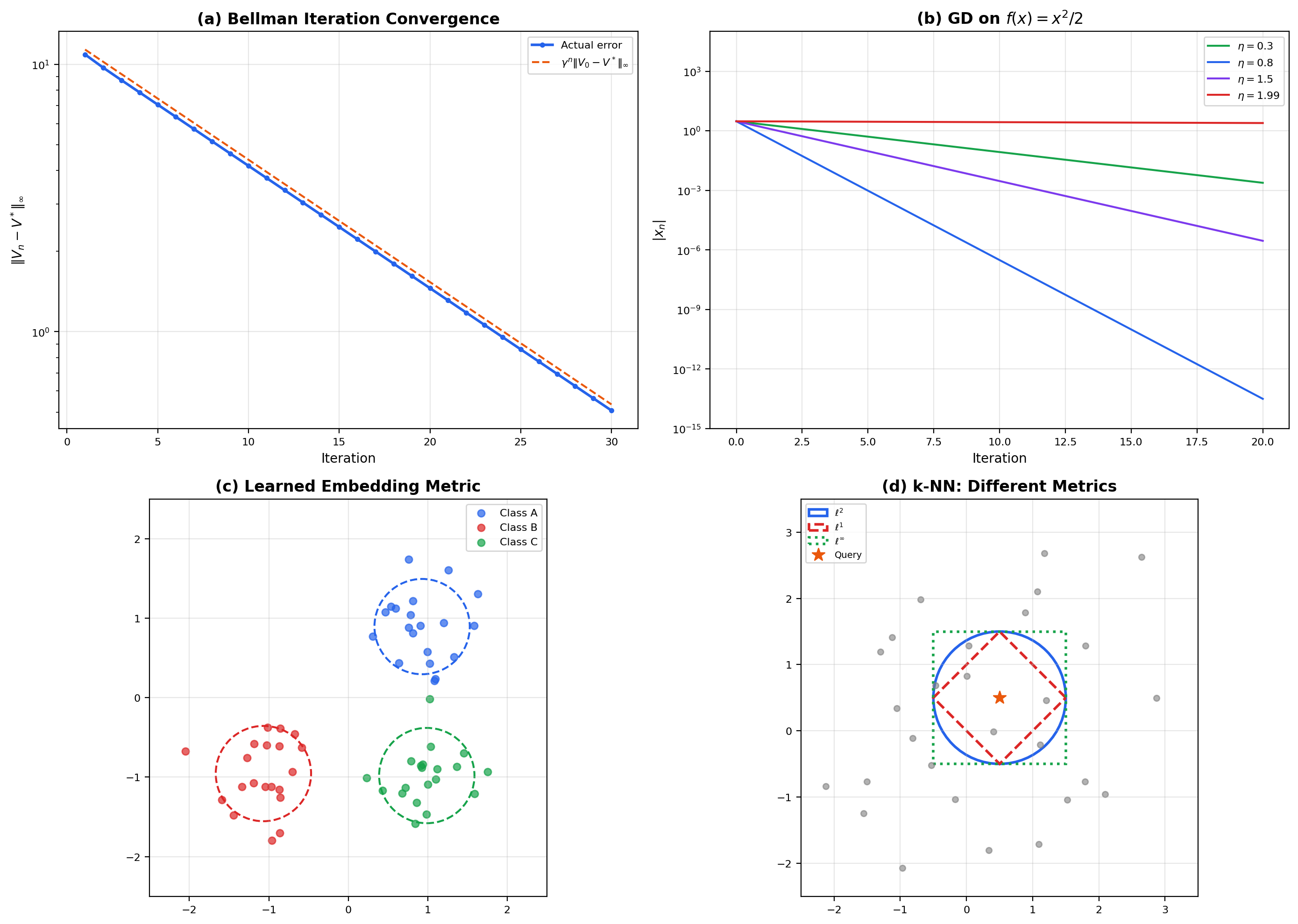
The proof is a short computation using the inequality and the fact that transition probabilities sum to 1. By Banach’s theorem, value iteration — the algorithm that repeatedly applies starting from any initial — converges to the unique optimal value function , at a geometric rate . This single fact is the reason value iteration works; it is also why a smaller discount (more aggressively short-sighted) gives faster convergence but different optimal policies. The viz below shows this concretely on a 3-state MDP.
Three states with two actions each. C is the reward-rich absorbing-ish state; the optimal policy is "move toward C then stay". The Bellman optimality operator T* is a γ-contraction in the sup-norm, so Banach's theorem guarantees V_n → V* at the geometric rate γⁿ.
📝 Example 15 (Lipschitz Continuity and Gradient Descent)
A function has -Lipschitz gradient if for all — the gradient map is Lipschitz with constant . For such functions, the gradient descent map has a Lipschitz constant of at most on an -strongly-convex function, which is strictly less than 1 whenever . So gradient descent is a contraction on strongly convex -smooth objectives, and the Banach theorem gives convergence to the unique minimizer at a geometric rate — this is the simplest known convergence proof for gradient descent. Much of convex optimization theory elaborates this idea: different step-size rules, accelerated methods, stochastic variants, and second-order methods all trade off against how tightly you can control the contraction constant.
📝 Example 16 (Metric Learning and Embedding Spaces)
Modern neural networks routinely learn metrics rather than using a fixed one. Three examples:
- Siamese networks learn an embedding and use as a learned similarity. The training objective forces the embedding to place semantically similar inputs close together.
- Triplet loss enforces for anchor , positive example , and negative example . The triangle inequality of the embedding metric constrains which triplet configurations are even geometrically possible, which is why well-trained embeddings exhibit the “tripletable” structure we see in Word2Vec and BERT representations.
- Contrastive learning (SimCLR, CLIP) implicitly learns a metric on the representation space where positive pairs are close and negative pairs are far, using cross-entropy loss as a surrogate for metric constraints.
In every case, the metric space axioms — positivity, symmetry, triangle inequality — are the constraints that well-behaved similarity scores must satisfy. A “distance” that violates symmetry () or the triangle inequality cannot be used with nearest-neighbor search acceleration structures like ball trees, and training losses that silently break the axioms often produce embedding spaces with weird pathologies.
💡 Remark 8 (k-NN and Metric Spaces)
The -nearest-neighbors algorithm is defined entirely in terms of a metric on the input space. Different metrics give different classifiers: Euclidean -NN, Manhattan -NN, Mahalanobis -NN, and cosine-similarity -NN all disagree on which points are “close” to a query. The triangle inequality is not just an axiom — it is what makes efficient nearest-neighbor search possible. Metric trees (ball trees, KD-trees, VP-trees) use the triangle inequality to prune branches of the search: if the distance from the query to a node’s center plus the node’s radius is larger than the best candidate found so far, the entire subtree can be skipped. Without the triangle inequality, no such pruning is correct, and nearest-neighbor search becomes linear in the dataset size. This is a concrete case where a mathematical axiom translates directly into algorithmic efficiency.
11. Computational Notes
Every concept in this topic has a short Python implementation. NumPy and SciPy have the basic machinery; the reference notebook spells out each one in detail.
distances in are a single NumPy call:
import numpy as np

def lp_distance(x, y, p=2):
    return np.linalg.norm(x - y, ord=p)

# Euclidean (p=2), Manhattan (p=1), Chebyshev (p=inf)
lp_distance(np.array([1, 2, 3]), np.array([4, 6, 8]), p=2)
Fixed-point iteration is a for-loop with a convergence check. For a contraction :
def fixed_point_iterate(T, x0, tol=1e-10, max_iter=1000):
    x = np.asarray(x0, dtype=float)
    for n in range(max_iter):
        x_new = T(x)
        if np.linalg.norm(x_new - x) < tol:
            return x_new, n + 1
        x = x_new
    return x, max_iter
The loop returns the iterate and the number of steps needed. Feed this a Picard operator, a Newton step, or a Bellman backup and the same skeleton applies.
Sup-norm distance between sampled functions is max(abs(...)) on a shared grid:
def sup_norm_distance(f_samples, g_samples):
    return np.max(np.abs(f_samples - g_samples))

x_grid = np.linspace(0, 1, 1000)
f = np.sin(2 * np.pi * x_grid)
g = np.sin(3 * np.pi * x_grid)
sup_norm_distance(f, g)
Pairwise distance matrices use scipy.spatial.distance.cdist, which supports every metric out of the box:
from scipy.spatial.distance import cdist

points = np.random.randn(100, 5)
D = cdist(points, points, metric='euclidean')  # or 'cityblock', 'chebyshev', ...
Value iteration on a small MDP is just repeated Bellman-optimality updates:
def value_iteration(P, R, gamma, tol=1e-10, max_iter=1000):
    # P: shape (S, A, S) transitions; R: shape (S, A) rewards
    S, A, _ = P.shape
    V = np.zeros(S)
    for n in range(max_iter):
        Q = R + gamma * P @ V  # shape (S, A)
        V_new = Q.max(axis=1)
        if np.max(np.abs(V_new - V)) < tol:
            return V_new, n + 1
        V = V_new
    return V, max_iter
The convergence rate matches the theoretical bound — you can verify this by plotting against and reading off the slope.
12. Summary and Key Results
The topic built a small library of theorems on top of the three metric-space axioms. Here is the proof-dependency structure in compact form.
| Result | Section | Key idea |
|---|---|---|
| Metric space axioms | 2 | Positivity, symmetry, triangle inequality |
| Three characterizations of continuity (Theorem 1) | 4 | ε–δ = sequential = preimage-of-open |
| Completeness of (Theorem 2) | 5 | Uniform limit of continuous is continuous |
| Compactness equivalence (Theorem 3) | 6 | Compact ⟺ sequentially compact ⟺ complete + totally bounded |
| Banach Contraction Mapping Theorem (Theorem 4) | 7 | Geometric-series Cauchy bound + completeness |
| Arzelà–Ascoli Theorem (Theorem 5) | 9 | Diagonal subsequence + equicontinuity promotes to uniform |
The dependency chain is linear. The compactness equivalence (Theorem 3) gives us the tools to recognize compactness without unrolling open covers every time. The completeness of (Theorem 2) is the missing ingredient for fixed-point arguments, and Theorem 2’s proof depends on the Uniform Limit Theorem from Uniform Convergence. The Banach theorem (Theorem 4) depends on completeness. Arzelà–Ascoli (Theorem 5) depends on completeness and on the compactness equivalence. All of these depend on the three characterizations of continuity from Theorem 1.
One result unifies four earlier topics. The Banach Contraction Mapping Theorem gives a single proof that covers:
- The Picard–Lindelöf existence theorem for first-order ODEs (Topic 21)
- Newton iteration for implicit numerical methods (Topic 24)
- The Inverse Function Theorem (Topic 12)
- Value iteration in reinforcement learning (Section 10)
Before this topic, each of those was a separate argument using a specifically constructed self-map. After this topic, they are four corollaries of one theorem about complete metric spaces — and the proof you read in Section 7 is the proof of all four at once.
13. Track 8 Opening — The Road to Functional Analysis
This topic opens Track 8: Functional Analysis Essentials, a four-topic arc that adds successively more structure to metric spaces until we reach the framework behind modern machine learning optimization. Each topic adds one layer:
Topic 29 (this topic): Metric Spaces & Topology. The language of distance, open sets, completeness, and compactness in abstract spaces. The Banach Contraction Mapping Theorem unifies convergence arguments across the curriculum. The Arzelà–Ascoli theorem characterizes compact function families. Forward-looking: this is the geometric foundation.
Topic 30: Normed & Banach Spaces. Add algebraic structure — a vector-space operation and a norm that interacts with it. Bounded linear operators replace generic continuous maps; the three pillars of functional analysis (Open Mapping, Closed Graph, Uniform Boundedness) emerge as consequences of the Baire Category Theorem we deferred from this topic. The payoff: “metric space + vector space = analysis powerhouse.” Dual spaces of linear functionals live here, and the spaces we have been quietly alluding to are Banach spaces — their theory gets its full treatment in Topic 30, not here.
Topic 31: Inner Product & Hilbert Spaces. Add geometric structure — an inner product that gives us angles, orthogonality, and projections. Orthogonal projections replace Banach-space linear functionals as the primary construction; the Riesz representation theorem identifies the dual of a Hilbert space with the space itself. This is the mathematical home of kernel methods, Reproducing Kernel Hilbert Spaces (RKHS), and Gaussian processes. Every symmetric positive-definite kernel in machine learning induces a Hilbert space; Topic 31 makes that construction rigorous.
Topic 32: Calculus of Variations. Optimization on function spaces. The Euler–Lagrange equations characterize critical points of functionals , first and second variation generalize the gradient and Hessian, and the direct method of the calculus of variations gives existence theorems via compactness arguments (Arzelà–Ascoli and its Sobolev-space cousins). This is the framework behind physics-informed neural networks, optimal transport, variational autoencoders, and diffusion models — wherever ML optimizes over functions rather than parameters, calculus of variations is quietly at work.
The refinement sequence is metric → normed → inner product → optimization. Every Hilbert space is a Banach space; every Banach space is a metric space. The additional structure at each step buys additional theorems: metric spaces give us continuity and contraction arguments, normed spaces add linear operators and duality, inner product spaces add orthogonal projection, and the optimization layer turns projection into the Euler–Lagrange machinery.
Connections & Further Reading
Prerequisites — topics you need first
Completeness & Compactness
Topic 3 established completeness and compactness in R^n via Bolzano-Weierstrass and Heine-Borel. Topic 29 generalizes both concepts to arbitrary metric spaces, resolving the C([0,1]) counterexample promised in Topic 3.
Uniform Convergence
Topic 4 introduced the sup-norm, equicontinuity, and previewed Arzelà-Ascoli. Topic 29 proves Arzelà-Ascoli in full and establishes C([a,b]) as a complete metric space under the sup-norm.
First-Order ODEs & Existence Theorems
Topic 21's Picard-Lindelöf existence theorem used a contraction argument on C([a,b]). Topic 29 proves the abstract Contraction Mapping Theorem that generalizes it.
Inverse & Implicit Function Theorems
Topic 12's proof of the Inverse Function Theorem used a contraction mapping argument. Topic 29 provides the abstract framework.
Numerical Methods for ODEs
Topic 24's convergence analysis of implicit methods invoked contraction mapping for Newton iteration. Topic 29 proves the general result.
Approximation Theory
Topic 20's density of polynomials in C[a,b] used the sup-norm metric. Topic 29 formalizes C([a,b]) as a complete metric space and connects density to the contraction mapping framework.
Line Integrals & Conservative Fields
Topic 15 mentioned simply connected domains and fundamental groups. Topic 29's general topology section provides the topological vocabulary for these concepts.
Where this leads — next in formalCalculus
Normed & Banach Spaces
Adds algebraic structure (vector space + norm) on top of the metric-space framework. The Baire Category Theorem, Open Mapping Theorem, Closed Graph Theorem, and Uniform Boundedness Principle — all deferred from this topic — are proved there.
Inner Product & Hilbert Spaces
Adds the inner-product structure that gives angles, orthogonality, the projection theorem, Riesz representation, and the RKHS construction behind kernel methods.
Calculus of Variations
The Euler-Lagrange equation, second variation, and the direct method for existence of minimizers via weak compactness. Arzelà-Ascoli from this topic reappears in Sobolev spaces as the compactness tool variational problems rely on.
On to formalStatistics — where this calculus powers inference
Empirical Processes
Donsker's theorem is a statement in the metric space D[0,1] with the Skorohod metric: √n(F_n - F) converges in distribution to the Brownian bridge. Continuity of functionals in this metric is what the continuous mapping theorem exploits.
Bayesian Computation And MCMC
Convergence rates of MCMC are metric-space statements: the chain converges to its stationary distribution in total-variation distance or Wasserstein distance. Contraction-mapping arguments (coupling) give geometric convergence rates.
On to formalML — where this calculus powers ML
References
- book Munkres, J. R. (2000). Topology Second edition. Chapters 2–3 (metric spaces, topological spaces, connectedness, compactness). The standard reference for general topology.
- book Rudin, W. (1976). Principles of Mathematical Analysis Third edition. Chapters 2–3 (basic topology, continuity). Clean treatment of metric-space compactness.
- book Folland, G. B. (1999). Real Analysis: Modern Techniques and Their Applications Second edition. Chapter 4 (point-set topology in analysis context). Good for the Arzelà–Ascoli proof.
- book Kreyszig, E. (1978). Introductory Functional Analysis with Applications Chapter 1 (metric spaces as foundation for functional analysis). Excellent pedagogy for the intermediate reader; Section 1.4 covers the contraction mapping theorem with worked examples.
- book Stein, E. M. & Shakarchi, R. (2005). Real Analysis: Measure Theory, Integration, and Hilbert Spaces Chapter 7 (Hausdorff measure, fractals). Peripheral to Topic 29 but useful for the general topology bridge.