Line Integrals & Conservative Fields
Integrating functions and vector fields along curves — the Gradient Theorem as the FTC for paths, conservative fields and potential functions, path independence, Green's theorem connecting circulation to double integrals, and gradient flow as continuous-time optimization.
Abstract. Line integrals extend integration from intervals and regions to curves. Given a parameterized curve C in ℝⁿ and a scalar function f, the scalar line integral ∫_C f ds = ∫_a^b f(r(t)) ‖r'(t)‖ dt sums f along C weighted by arc length. Given a vector field F, the vector line integral (work integral) ∫_C F · dr = ∫_a^b F(r(t)) · r'(t) dt measures the total work done by F along C. A vector field F is conservative if F = ∇f for some potential function f. The Gradient Theorem — the Fundamental Theorem of Calculus for line integrals — states that ∫_C ∇f · dr = f(r(b)) − f(r(a)): the integral depends only on the endpoints, not the path. This is equivalent to path independence: the integral of a conservative field between two points is the same regardless of which curve connects them. In ℝ², the exactness criterion ∂P/∂y = ∂Q/∂x characterizes conservative fields on simply connected domains. On domains with holes, closed fields need not be exact — the topology of the domain matters, as demonstrated by the vortex field. Green's theorem provides the bridge between line integrals and double integrals: the circulation ∮_C F · dr around a closed curve equals the double integral ∬_D (∂Q/∂x − ∂P/∂y) dA over the enclosed region. The integrand is the 2D curl of F, measuring infinitesimal rotation. Green's theorem also yields the area formula A = ½ ∮_C (x dy − y dx). In machine learning, gradient flow dθ/dt = −∇L(θ) traces a curve in parameter space along which the loss decreases monotonically — the Gradient Theorem guarantees L(θ(T)) − L(θ(0)) = −∫₀ᵀ ‖∇L(θ(t))‖² dt ≤ 0. Energy-based models define a scalar potential whose gradient field governs the model's dynamics. The natural gradient follows geodesics on the statistical manifold rather than straight lines in parameter space.
1. Overview & Motivation
You’re training a neural network. At each step, gradient descent moves the parameter vector a small distance in the direction . Over many steps, the parameters trace a curve through parameter space — a winding path from initialization to (hopefully) a minimum. How much does the loss decrease along that entire path?
The answer is a line integral: . The Gradient Theorem — the subject of this topic — says this integral equals , regardless of the path’s shape. This is the Fundamental Theorem of Calculus, generalized from intervals to curves in .
But not every vector field is a gradient. When a field is a gradient — when it is conservative — integration becomes dramatically simpler: the integral depends only on the endpoints, not the path. When a field is not conservative, the path matters, and the distinction between “conservative” and “not conservative” becomes a topological question about the domain. That question — when does the shape of the path matter? — is the central thread of this topic.
2. Parameterized Curves
Before we can integrate along curves, we need to say precisely what a “curve” is and how to measure length along it.
A curve in is a path traced out by a moving point. We describe it by giving the position at each “time” : the parameterization for . The velocity vector points along the curve, and its magnitude is the speed. Arc length — the total distance traveled — is the integral of speed.
📐 Definition 1 (Parameterized Curve)
A parameterized curve in is a continuous function . The curve is smooth if is and for all — the velocity never vanishes, so the particle never stops. The curve is piecewise smooth if can be partitioned into finitely many subintervals on each of which is smooth.
📐 Definition 2 (Arc Length)
The arc length of a smooth curve is
The arc length element is , representing the infinitesimal distance traveled in an infinitesimal time .
💡 Remark 1 (Reparameterization Invariance)
If is a bijection with (orientation-preserving), then traces the same curve in the same direction. By the substitution rule (Topic 14, Theorem 1):
Arc length does not depend on how fast we traverse the curve — it is a geometric property of the curve itself.
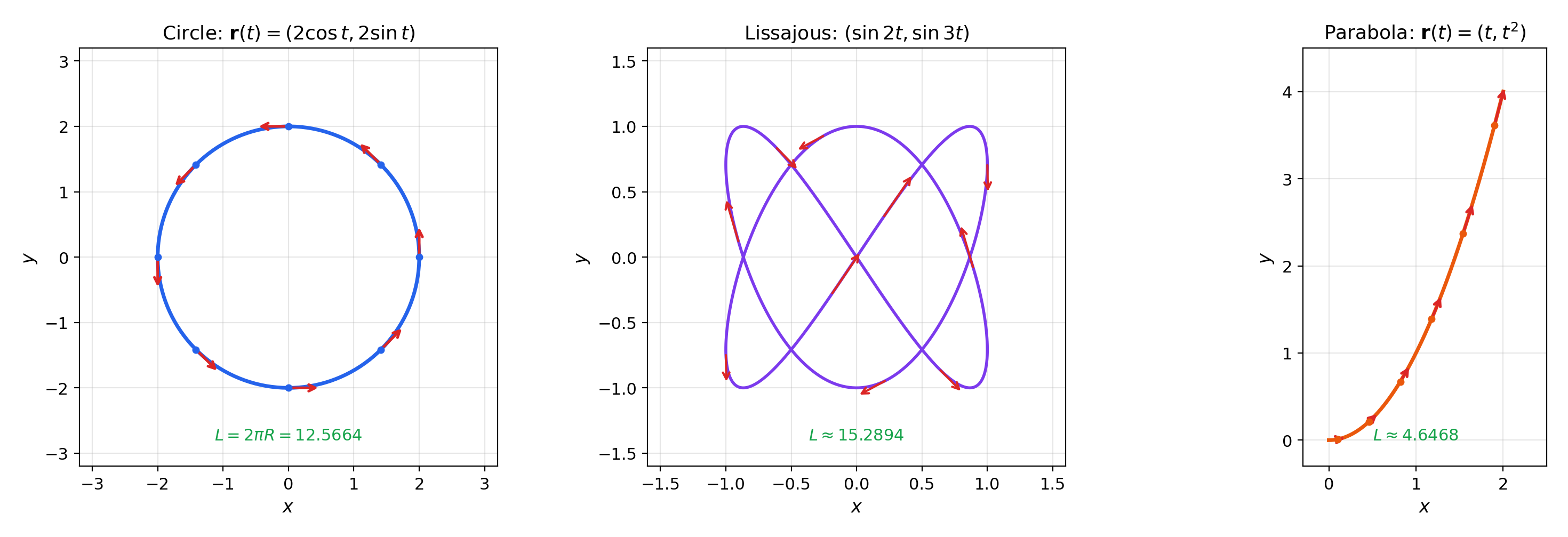
📝 Example 1 (Circle of Radius R)
Let for . Then and . The arc length is
The constant speed means the particle moves uniformly — the arc length is simply speed times time.
📝 Example 2 (Helix)
A helix for climbs one full turn. We have , giving . The vertical climb adds length to the horizontal circle.
📝 Example 3 (Parabolic Arc)
The parabola for has . The arc length integral requires the formula or numerical quadrature — not every arc length computation is elementary.
3. Scalar Line Integrals
The scalar line integral sums the values of a function along a curve , weighted by arc length. If , we recover the arc length itself. If represents density (mass per unit length), the integral gives total mass.
Imagine a wire bent into the shape of , with density at each point. The total mass is . The wire analogy makes clear why we weight by rather than : the physical mass depends on the curve’s geometry, not on how fast we parameterize it.
📐 Definition 3 (Scalar Line Integral)
Let be a smooth curve parameterized by , and let be continuous. The scalar line integral of over is:
This is a Riemann integral (Topic 7) of the composite function over .
🔷 Proposition 1 (Parameterization Independence)
The scalar line integral is independent of the parameterization of (including orientation). Any two smooth parameterizations of the same curve give the same value.
Proof.
Let and with a bijection. By the chain rule, , so . Then:
By the substitution rule (Topic 14, Theorem 1) with , this equals . The absolute value ensures the result holds regardless of whether preserves or reverses orientation.
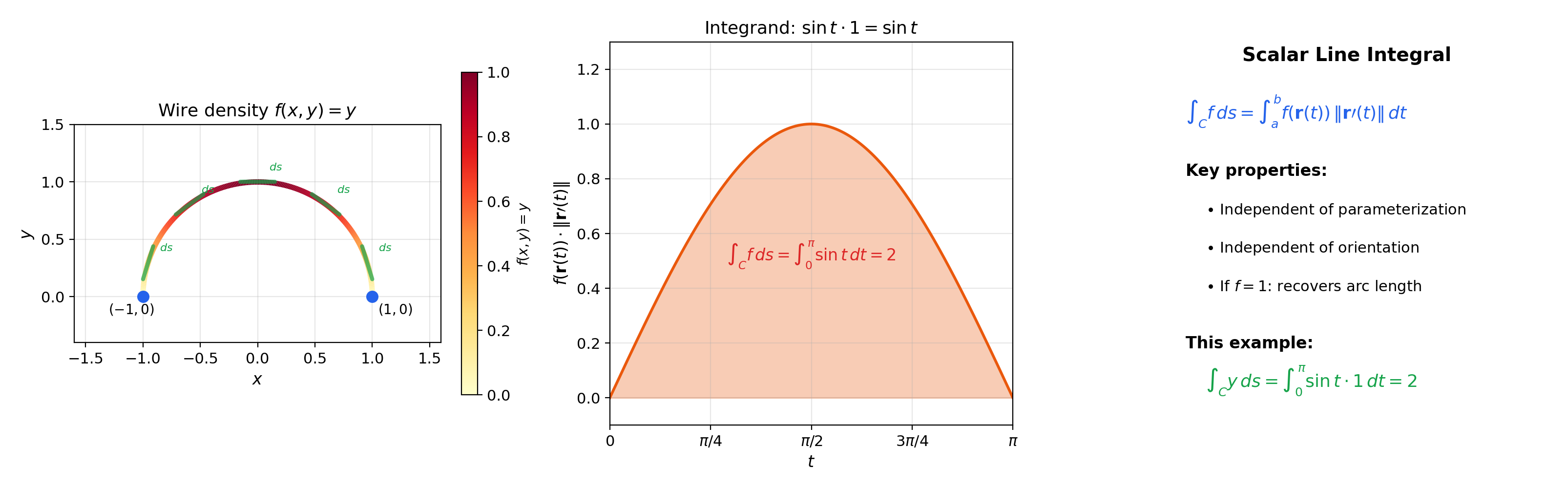
📝 Example 4 (Mass of a Semicircular Wire)
A wire follows for with density . Then:
The wire is heaviest at the top () and weightless at the endpoints (). The total mass is 2.
📝 Example 5 (Average Value Along a Curve)
The average value of over is , directly analogous to from single-variable calculus (Topic 7).
4. Vector Line Integrals — The Work Integral
The vector line integral measures the work done by a force field on a particle moving along . Unlike the scalar line integral, this integral is orientation-sensitive — reversing the direction of traversal negates the result.
At each point on , the vector field has a component tangent to the curve and a component perpendicular to it. Only the tangent component contributes to work. The dot product extracts exactly this tangent component (times the speed). Integrating over sums up the infinitesimal contributions along the entire path.
📐 Definition 4 (Vector Line Integral)
Let be a smooth curve parameterized by and a continuous vector field. The vector line integral (or work integral) of along is:
In , writing and , this becomes .
💡 Remark 2 (Orientation Matters)
Reversing the curve — traversing from to — negates the integral: . This is because reverses sign under orientation reversal, and the dot product is linear. By contrast, the scalar line integral is orientation-independent because is always positive.
💡 Remark 3 (Parameterization Independence)
The vector line integral is independent of the orientation-preserving parameterization. Any two parameterizations that traverse in the same direction yield the same value. The proof is the same substitution argument as Proposition 1, but without the absolute value — the sign of cancels the reversed limits, preserving the integral’s value.
🔷 Theorem 1 (Properties of Line Integrals)
Let , , be piecewise-smooth curves, , continuous vector fields, and .
-
Linearity: .
-
Additivity over path concatenation: If (the endpoint of is the start of ), then .
-
Orientation reversal: .
📝 Example 6 (Work by a Constant Force)
Let and be the line segment from to : for . Then and:
For a constant field, the work equals — the integral is just a dot product.
📝 Example 7 (Work by a Radial Field)
Let and be the upper semicircle from to : for . Then :
The radial field is everywhere perpendicular to the circle — it does zero work along any circular arc.
📝 Example 8 (Work by a Non-Conservative Field)
Let . Compute the work along two different paths from to :
Path : Line segment for . Then and :
Path : Quarter-circle for . Then :
Different paths, different integrals (). This field is not conservative.
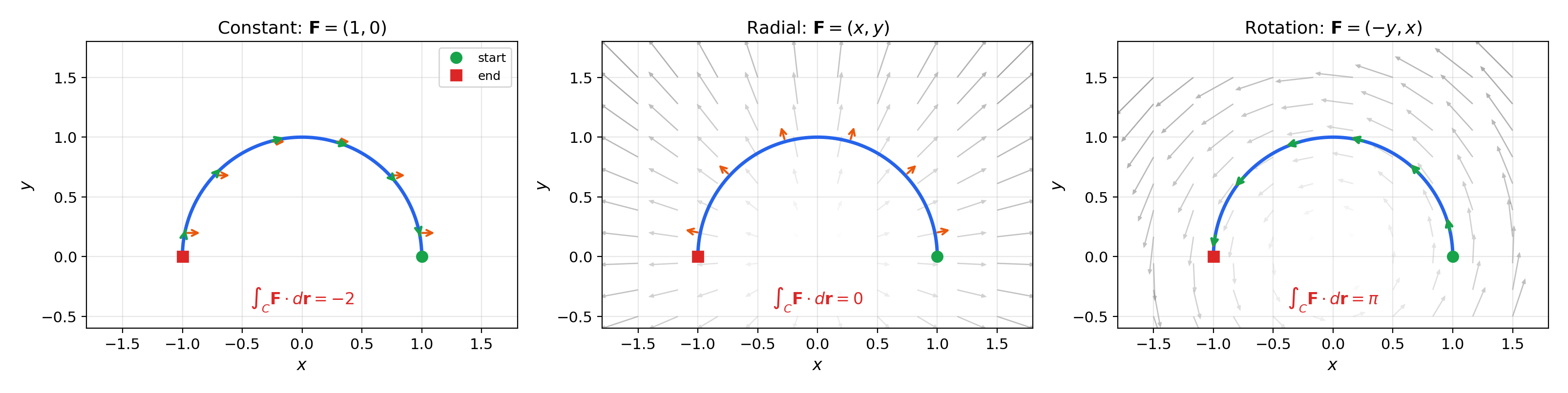
Rigid counterclockwise rotation. Constant curl = 2 everywhere.
5. Conservative Fields & the Gradient Theorem
This section contains the most important result in the topic — the Fundamental Theorem of Calculus for line integrals. It explains why “gradient” and “conservative” are the same concept.
If , then the work integral is just the total change in along the curve — the difference between the “heights” at the endpoints. Think of as elevation: a hiker following a trail gains elevation regardless of the trail’s shape. The gradient field always points uphill, so walking along a contour (level curve of ) does zero work — the gradient is perpendicular to level sets (Topic 9).
📐 Definition 5 (Conservative Vector Field)
A vector field (where is open and connected) is conservative if there exists a function such that on . The function is called a potential function (or scalar potential) for .
💡 Remark 4 (Potential Functions Are Unique Up to a Constant)
If and are both potential functions for on a connected domain , then on , so is constant. This follows from the fact that a function with zero gradient on a connected domain must be constant — a consequence of the Mean Value Theorem (Topic 6).
🔷 Theorem 2 (The Gradient Theorem (FTC for Line Integrals))
Let be a function on an open set , and let be a piecewise-smooth curve in from to . Then:
Proof.
Define for . By the chain rule (Topic 5 for scalar functions, Topic 10 for the multivariable version):
This is the key identity: the integrand of the line integral is exactly . By the Fundamental Theorem of Calculus (Topic 7, Theorem 2):
The proof is strikingly short — it’s the chain rule plus the FTC. The chain rule converts the multivariable line integral into a single-variable integral, and the FTC evaluates it. This is why the Gradient Theorem is the “FTC for line integrals.”
📝 Example 9 (Gravitational Potential)
Let with potential . For any curve from to :
No parameterization needed — just endpoint evaluation.
📝 Example 10 (Verifying Example 7 via the Gradient Theorem)
The radial field . The curve from to gives:
The Gradient Theorem reproduces Example 7’s result — zero work — without any integration.
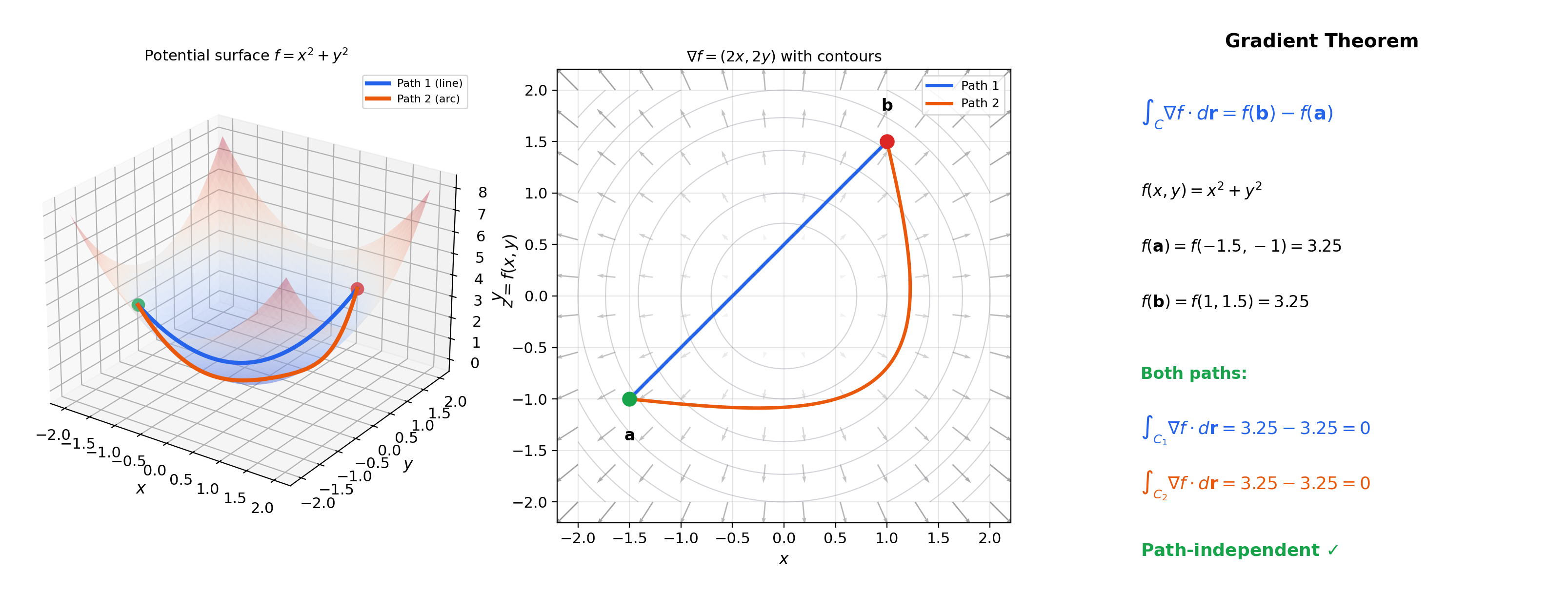
The surface shows φ(x, y). The gradient field ∇φ is projected onto the floor plane. For any curve C from point A to point B, the Gradient Theorem gives ∫C ∇φ · dr = φ(B) − φ(A).
6. Path Independence & the Exactness Criterion
When is a vector field conservative? The Gradient Theorem shows that conservative fields have path-independent integrals. The converse is also true: path independence implies conservativeness. And there is a practical, computable test.
📐 Definition 6 (Path Independence)
A vector field has path-independent line integrals if for every pair of piecewise-smooth curves in that share the same endpoints.
📐 Definition 7 (Closed Curve)
A curve parameterized by is closed if . We write for integrals over closed curves.
🔷 Theorem 3 (Equivalence of Conservative, Path-Independent, and Zero-Circulation)
Let be a continuous vector field on an open connected domain . The following are equivalent:
- is conservative ( for some function ).
- is path-independent in .
- for every piecewise-smooth closed curve in .
Proof.
(1) (2): Immediate from the Gradient Theorem — the integral equals , which depends only on the endpoints.
(2) (3): If is closed, its start and end points coincide: . Split at any interior point into two curves (from to ) and (from to ). By path independence, , so .
(3) (1): Fix a base point and define where is any path from to . The zero-circulation condition ensures this is well-defined (different paths give the same value).
To show : compute by choosing the path to as any path from to , then a straight segment from to . The difference . By the FTC (Topic 7), dividing by and taking gives .
📐 Definition 8 (Simply Connected Domain)
An open connected domain is simply connected if every closed curve in can be continuously shrunk to a point without leaving . Informally: has no holes. The full plane is simply connected; the punctured plane is not.
🔷 Theorem 4 (Exactness Criterion)
Let be a vector field on an open, simply connected domain . Then is conservative if and only if:
💡 Remark 5 (Why 'Simply Connected'?)
The condition says is closed — its 1-form is closed. On simply connected domains, closed = exact (= conservative). On domains with holes, closed exact. The gap is topological, not analytical — it is measured by de Rham cohomology (→ Smooth Manifolds on formalML).
📝 Example 11 (Testing Conservativeness)
Let . Check: . Conservative.
Find : from we get . Then forces , so .
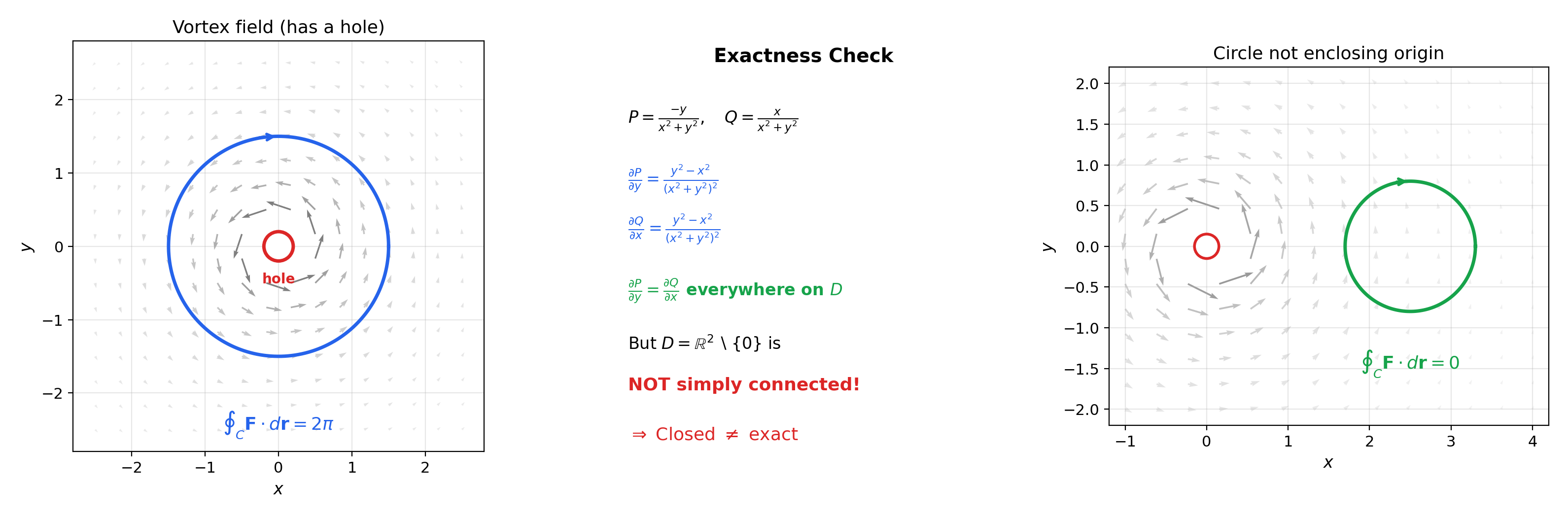
📝 Example 12 (The Vortex Field — Topology Matters)
The vortex field on .
Check the exactness condition: . The condition holds, yet the circulation around the unit circle is:
The catch: is not simply connected — it has a hole at the origin. The “potential function” is multi-valued; it gains each time we circle the origin. The vortex field is the canonical example showing that topology matters.
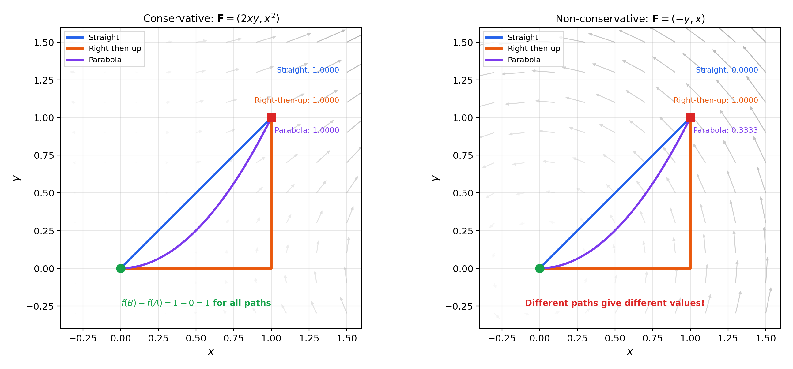
Conservative field
| Straight line | 1.5000 |
| Parabolic arc | 1.5000 |
| Circular arc | 1.5000 |
All paths give the same value
Non-conservative field
| Straight line | 0.0000 |
| Parabolic arc | 0.7500 |
| Circular arc | 1.2843 |
Different paths, different values
7. Green’s Theorem
Green’s theorem converts a line integral around a closed curve into a double integral over the enclosed region. This is the 2D special case of the generalized Stokes’ theorem — the single most powerful identity in vector calculus.
Walk around the boundary of a region . At each point, the vector field pushes you along (or against) your direction of travel. The total work around the loop — the circulation — equals the integral of the “rotation” of over the interior. That “rotation” is , the 2D curl.
🔷 Theorem 5 (Green's Theorem)
Let be a bounded region with piecewise-smooth boundary oriented counterclockwise. Let be a vector field. Then:
Proof.
We show and separately, then add.
Proof that : Let be a Type I region: , . The right side is:
The boundary traversed counterclockwise consists of: the bottom curve from to , the right side, the top curve from to , and the left side. On : . On (reversed): . On the vertical sides, , so their contributions vanish. Adding:
The proof for is analogous using a Type II description of . For general regions, decompose into Type I and Type II pieces; interior boundary contributions cancel in pairs.
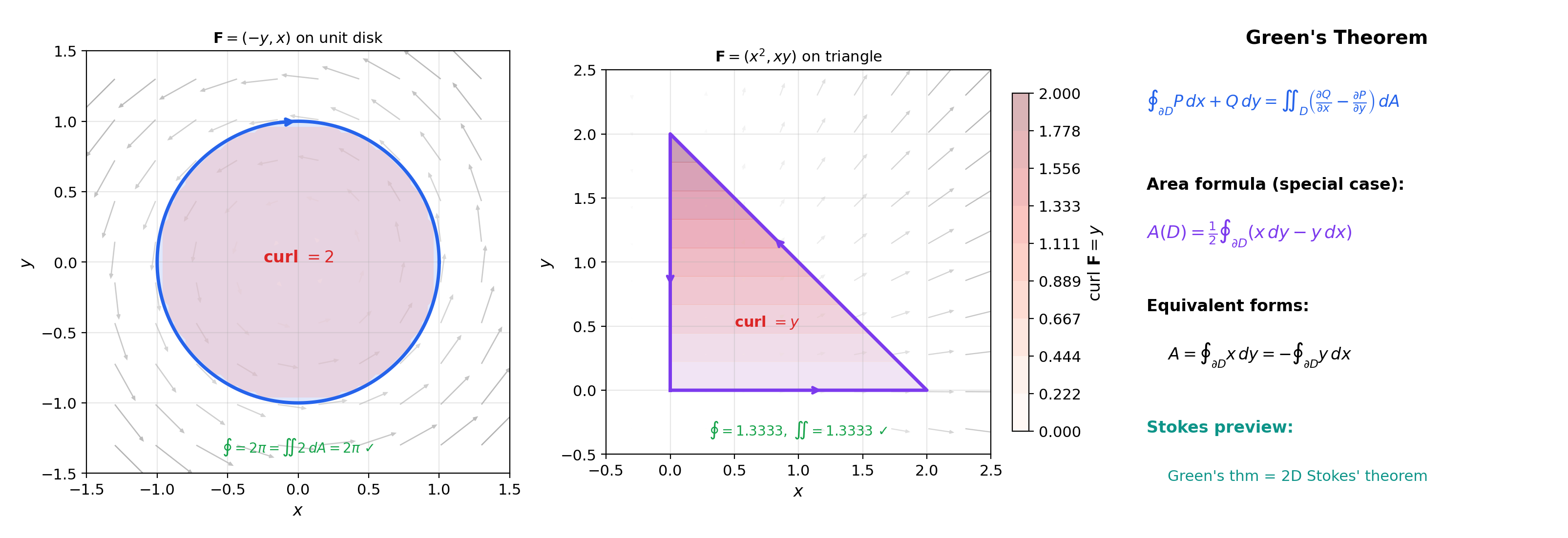
📝 Example 13 (Circulation of F = (−y, x) Around the Unit Circle)
Direct computation: with gives:
Via Green’s theorem: , so:
Both give . The rotation field has constant curl 2 — every point in the disk contributes equally to the circulation.
📝 Example 14 (Area via Green's Theorem)
Setting , gives , so:
This is the Shoelace formula for polygonal areas (a special case when is a polygon) and the formula used by mechanical planimeters.
💡 Remark 6 (Green's Theorem as a Conservation Law)
Green’s theorem says that the “total rotation inside ” equals the “total circulation around .” The interior quantity (curl) and the boundary quantity (circulation) are related by an exact balance. This is the prototype of all conservation laws in physics — and the 2D instance of Stokes’ theorem, which will be generalized to surfaces and volumes in Surface Integrals & the Divergence Theorem.
8. Curl & Circulation
The integrand in Green’s theorem — — is the 2D curl. It measures how much the vector field “rotates” around each point. We can formalize this by taking a limit of circulations over shrinking loops.
📐 Definition 9 (2D Curl (Scalar Curl))
For of class , the 2D curl (or scalar curl) is:
This is the -component of the 3D curl , with viewed as the 3D field .
🔷 Proposition 2 (Curl as Infinitesimal Circulation)
Let be at , and let be the circle of radius centered at , oriented counterclockwise. Then:
The curl is the circulation per unit area in the limit of infinitesimally small loops.
Proof.
By Green’s theorem, . By the Mean Value Theorem for double integrals (Topic 13), for some . As , and continuity of gives the limit.
💡 Remark 7 (Conservative ⟺ Curl-Free (on Simply Connected Domains))
Theorem 4 restated: on a simply connected domain, is conservative if and only if everywhere. Green’s theorem explains why: if on , then for every closed curve bounding a region in . On simply connected domains, every closed curve bounds a region in , so the zero-circulation condition (Theorem 3) is satisfied.
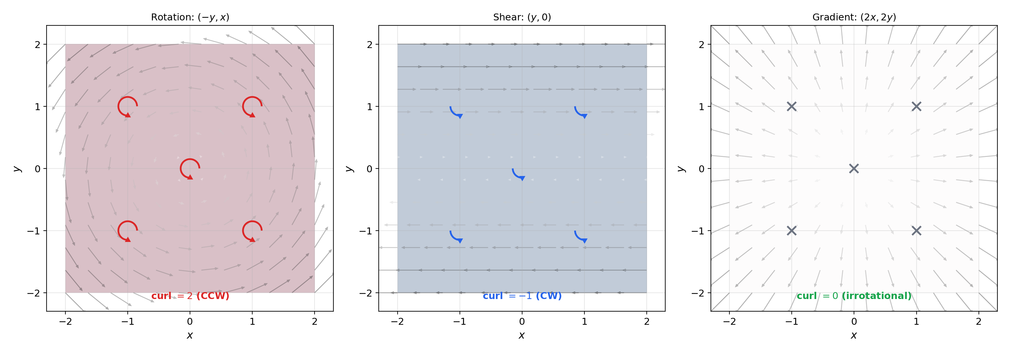
📝 Example 15 (Identifying Rotation)
Three vector fields, three curl values:
- Rotation field : . Constant positive curl — rigid counterclockwise rotation.
- Shear field : . Constant negative curl — clockwise shearing.
- Expansion field : . Curl-free — pure expansion, no rotation. This field is conservative (it’s a gradient field).
Drag to move the probe circle. As the radius shrinks, ∮/πr² → curl(F) at the center.
9. Computational Notes
In practice, line integrals are computed by reducing to single-variable integrals via parameterization, then applying numerical quadrature. Here are the key patterns:
Computing given and :
import numpy as np
from scipy.integrate import quad

def line_integral_vector(F, r, r_prime, a, b):
    """Compute ∫_C F · dr via parameterization."""
    def integrand(t):
        x, y = r(t)
        Fx, Fy = F(x, y)
        dx, dy = r_prime(t)
        return Fx * dx + Fy * dy
    result, _ = quad(integrand, a, b)
    return result
Testing conservativeness via finite differences:
def is_conservative(F, domain, grid_size=50, tol=1e-6):
    """Check ∂P/∂y ≈ ∂Q/∂x on a grid."""
    h = 1e-7
    xs = np.linspace(*domain[0], grid_size)
    ys = np.linspace(*domain[1], grid_size)
    max_dev = 0
    for x in xs:
        for y in ys:
            dP_dy = (F(x, y + h)[0] - F(x, y - h)[0]) / (2 * h)
            dQ_dx = (F(x + h, y)[1] - F(x - h, y)[1]) / (2 * h)
            max_dev = max(max_dev, abs(dQ_dx - dP_dy))
    return max_dev < tol
Recovering a potential function:
def find_potential(F, x, y):
    """Recover φ(x,y) by integrating along L-shaped path from (0,0)."""
    # Horizontal: ∫₀ˣ P(s, 0) ds
    phi_x, _ = quad(lambda s: F(s, 0)[0], 0, x)
    # Vertical: ∫₀ʸ Q(x, s) ds
    phi_y, _ = quad(lambda s: F(x, s)[1], 0, y)
    return phi_x + phi_y
Verifying Green’s theorem numerically:
# Line integral around unit circle
circulation = line_integral_vector(
    F=lambda x, y: (-y, x),
    r=lambda t: (np.cos(t), np.sin(t)),
    r_prime=lambda t: (-np.sin(t), np.cos(t)),
    a=0, b=2 * np.pi
)  # → 2π

# Double integral of curl over unit disk
from scipy.integrate import dblquad
curl_integral, _ = dblquad(
    lambda y, x: 2,  # curl = 2 everywhere
    -1, 1,
    lambda x: -np.sqrt(1 - x**2),
    lambda x: np.sqrt(1 - x**2)
)  # → 2π
10. Connections to ML
Line integrals appear in machine learning in three distinct ways. These are not afterthoughts — they are the mathematical backbone of how optimization, energy models, and natural gradients work.
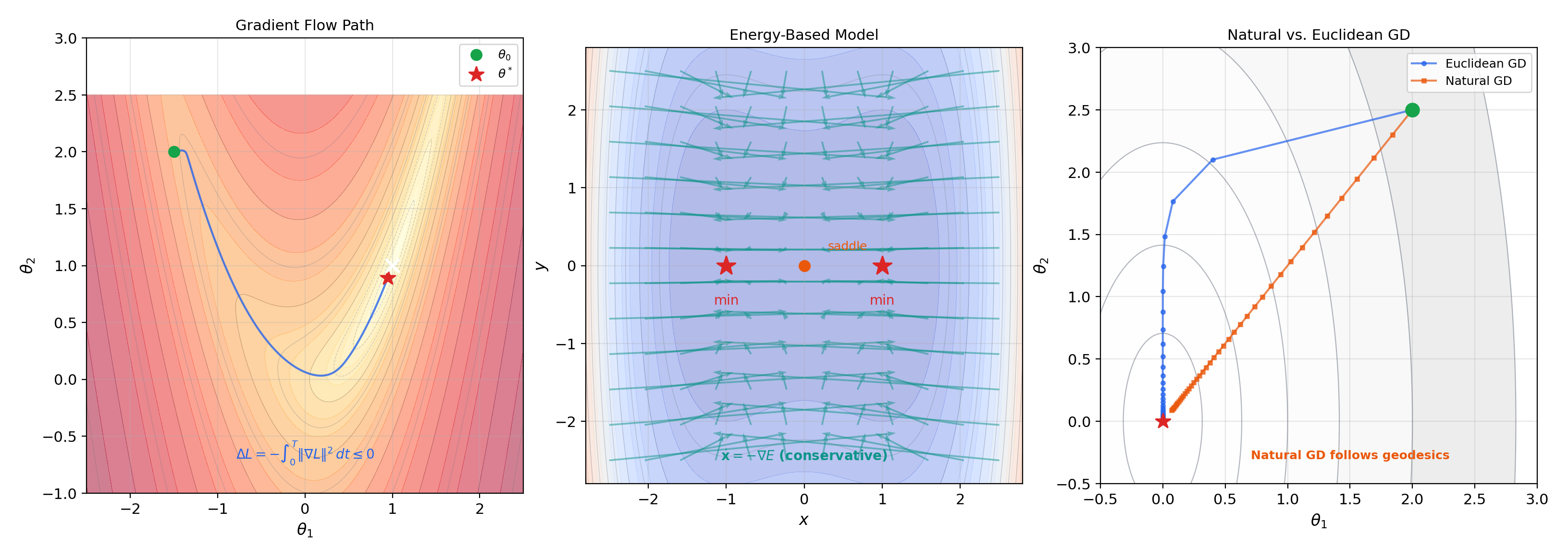
10.1 Gradient Flow as Continuous-Time Gradient Descent
The ODE defines a curve in parameter space. The total loss change along this curve is:
The first equality is the chain rule; the second substitutes . The integral is the “total gradient magnitude” along the path — it quantifies how much the loss decreases. This is the Gradient Theorem (Theorem 2) applied to , giving the loss difference as a line integral of .
Discrete gradient descent approximates this flow. The step size controls how closely the discrete path follows the continuous one. When is small, the discrete path stays near the continuous flow, and convergence analysis borrows from the continuous theory.
→ Gradient Descent on formalML
10.2 Energy-Based Models
An energy-based model defines a scalar potential over input space. The negative gradient pushes inputs toward low-energy configurations. The dynamics are a gradient flow in input space — a conservative system where the “work done” on equals the energy change , independent of path. Hopfield networks, Boltzmann machines, and score-based diffusion models all define energy landscapes whose gradient fields govern inference and generation.
10.3 Natural Gradient & Geodesic Paths
Standard gradient descent follows the direction in Euclidean parameter space. The natural gradient follows , where is the Fisher information matrix. This corresponds to steepest descent in the Fisher-Rao metric on the statistical manifold — the direction that maximally decreases the loss per unit of statistical distance.
The length of a curve in the Fisher-Rao metric is:
This is a scalar line integral (Definition 3) with the arc length element of the Fisher-Rao metric replacing the Euclidean one. Geodesics are curves that minimize this length integral — the calculus of variations provides the Euler-Lagrange equation for finding them.
→ Information Geometry on formalML
Connections & Further Reading
Prerequisites — topics you need first
Multiple Integrals & Fubini's Theorem
Green's theorem converts a line integral around a closed curve into a double integral over the enclosed region. The double integral machinery from Topic 13 — Fubini, Type I/II regions, iterated integration — is applied directly.
Partial Derivatives & the Gradient
The gradient ∇f is the engine of conservative fields. The Gradient Theorem is the direct connection: ∫_C ∇f · dr = f(b) − f(a). The gradient's orthogonality to level sets (Topic 9) explains why work integrals along level curves vanish.
The Derivative & Chain Rule
The Fundamental Theorem of Calculus (Topic 7, via Topic 5) has a direct analog: the Gradient Theorem is the FTC for line integrals. The chain rule d/dt f(r(t)) = ∇f(r(t)) · r'(t) is the key step in its proof.
The Jacobian & Multivariate Chain Rule
The multivariate chain rule J_{f∘g} = J_f · J_g (Topic 10) generalizes the chain rule step in the Gradient Theorem proof to vector-valued functions. The Jacobian framework clarifies why ∫_C F · dr is parameterization-independent.
Epsilon-Delta & Continuity
Continuity of F along the curve and continuity of r'(t) are the hypotheses that make the Riemann sum definition of the line integral well-defined. The limit of the approximating sums exists by the same uniform continuity argument as Topic 7.
Completeness & Compactness
Compactness of the curve image r([a,b]) ensures that continuous vector fields are bounded on C and that the line integral is well-defined as a finite number.
The Riemann Integral & FTC
After parameterization, every line integral reduces to a single-variable Riemann integral ∫_a^b g(t) dt. The existence and properties of line integrals follow from the 1D theory in Topic 7.
Where this leads — next in formalCalculus
Surface Integrals & the Divergence Theorem
Stokes' theorem generalizes Green's theorem from 2D to 3D: ∮_C F · dr = ∬_S (∇ × F) · dS. The divergence theorem relates surface integrals to volume integrals.
First-Order ODEs & Existence Theorems
Exact differential equations M dx + N dy = 0 are exact when M_y = N_x — the same criterion as conservative fields. The integrating factor technique corresponds to finding a potential function.
Metric Spaces & Topology
The topological vocabulary — open sets, continuity via preimages, homeomorphism, fundamental groups — underlies simply connected vs. non-simply-connected domains and the topological obstruction to conservativeness.
Calculus of Variations
Functionals J[γ] = ∫_a^b L(γ, γ', t) dt are line integrals over path space. Extremal paths satisfy the Euler-Lagrange equation — the direct descendant of this topic's variational structure.
On to formalML — where this calculus powers ML
Gradient Descent
Gradient flow dθ/dt = −∇L(θ) traces a curve in parameter space. The Gradient Theorem gives L(θ(T)) − L(θ(0)) = −∫₀ᵀ ‖∇L‖² dt ≤ 0, proving the loss decreases monotonically along the flow. Discrete gradient descent approximates this continuous path, and the integral quantifies convergence.
Smooth Manifolds
Line integrals are integrals of differential 1-forms ω = P dx + Q dy along curves. Conservative fields are exact forms (ω = df). The gap between closed and exact forms — measured by de Rham cohomology H¹ — is the topological obstruction to conservativeness. Green's theorem is the 2D Stokes' theorem.
Information Geometry
Geodesics on the statistical manifold minimize the Fisher-Rao length functional — a line integral of the metric tensor. The natural gradient follows these geodesics, and path length in the Fisher-Rao metric measures statistical distinguishability.
References
- book Spivak (1965). Calculus on Manifolds Chapter 4 — integration on chains, Stokes' theorem in the language of differential forms
- book Hubbard & Hubbard (2015). Vector Calculus, Linear Algebra, and Differential Forms Chapter 6 — line integrals, conservative fields, Green's theorem with geometric exposition
- book Munkres (1991). Analysis on Manifolds Chapter 5 — line integrals and Green's theorem with rigorous measurability conditions
- book Schey (2005). Div, Grad, Curl, and All That Chapters 2-3 — physical motivation for line integrals via work, circulation, and flux
- book Rudin (1976). Principles of Mathematical Analysis Chapter 10 — differential forms and Stokes' theorem in Rⁿ
- paper LeCun, Chopra, Hadsell, Ranzato & Huang (2006). “A Tutorial on Energy-Based Learning” Energy functions as potential functions whose gradient fields govern model dynamics
- paper Amari (1998). “Natural Gradient Works Efficiently in Learning” The natural gradient as a geodesic direction on the statistical manifold — line integral of the Fisher information metric