First-Order ODEs & Existence Theorems
Equations where the unknown is a function — direction fields, separation of variables, integrating factors, and the Picard-Lindelöf theorem that guarantees solutions exist and are unique when the right-hand side is Lipschitz.
Abstract. A first-order ordinary differential equation y' = f(t, y) asks: which function y(t) has the property that its derivative at every point equals f(t, y(t))? Direction fields visualize the answer geometrically — at every point (t, y), draw a short line segment with slope f(t, y), and the solution curves are the paths that follow these slopes. For separable equations y' = g(t)h(y), the variables can be separated and integrated independently. For linear equations y' + p(t)y = q(t), the integrating factor μ(t) = exp(∫p(t)dt) converts the left side into an exact derivative. For exact equations M dt + N dy = 0 with M_y = N_t, the solution is a level curve of a potential function — the same structure as conservative vector fields. The Picard-Lindelöf theorem guarantees that if f is continuous and Lipschitz in y, then the initial value problem y' = f(t, y), y(t₀) = y₀ has a unique local solution. The proof is constructive: the Picard iterates y_{n+1}(t) = y₀ + ∫f(s, yₙ(s))ds form a contraction mapping in the space of continuous functions, converging to the unique solution — the same fixed-point technique that proved the Inverse Function Theorem. When the Lipschitz condition fails, as in y' = y^{2/3}, existence (Peano) still holds, but uniqueness fails — solutions can branch. In machine learning, gradient descent is a discretized ODE: the continuous gradient flow θ̇ = −∇L(θ) is a first-order ODE whose solutions are guaranteed by Picard-Lindelöf when the loss landscape is smooth. Neural ODEs (Chen et al. 2018) replace discrete layers with continuous dynamics, using ODE solvers for the forward pass and the adjoint method for backpropagation.
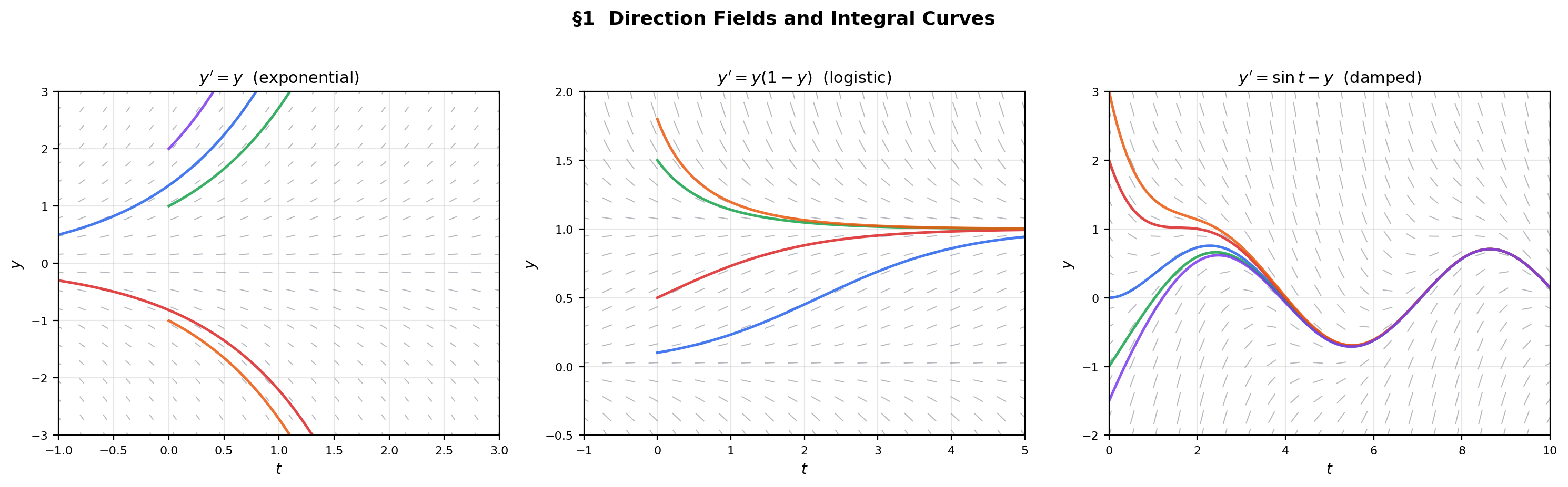
1. Direction Fields — The Geometry of an ODE
Until now, every equation we have solved has asked for a number: find such that , or find the value . An ordinary differential equation asks for something fundamentally different — a function. The equation asks: which function has the property that its derivative at every point equals ?
Before any algebra, we draw. A first-order ODE assigns a slope to every point in the plane. A direction field (also called a slope field) draws a short line segment at each point with the assigned slope. A solution is a curve that is tangent to the direction field at every point — an integral curve that threads through the field.
📐 Definition 1 (Ordinary Differential Equation (First-Order))
A first-order ordinary differential equation (ODE) is an equation of the form
where is a given function on an open set , and is the unknown function defined on an interval . The variable is the independent variable (often representing time), is the dependent variable (the state), and is the right-hand side (the vector field, in 1D).
📐 Definition 2 (Initial Value Problem)
An initial value problem (IVP) is an ODE together with an initial condition:
where is the specified starting point. A solution is a differentiable function (with ) satisfying both the equation and the initial condition.
📐 Definition 3 (Direction Field and Integral Curve)
The direction field of is the assignment — a line element of slope at each point. An integral curve is a curve that is tangent to the direction field at every point, i.e., .
📝 Example 1 (Exponential growth)
Consider with . The direction field has slope at : horizontal along , steeper as increases. Solutions are — exponentials that grow away from the equilibrium . Each initial condition determines a unique integral curve.
💡 Remark 1 (Direction fields vs. gradient fields)
The direction field of is a 1D analog of the gradient field from The Gradient & Directional Derivatives. Gradient descent is a first-order ODE whose direction field is . The integral curves are the gradient descent trajectories. This is not an analogy — it is literally the same mathematical structure.
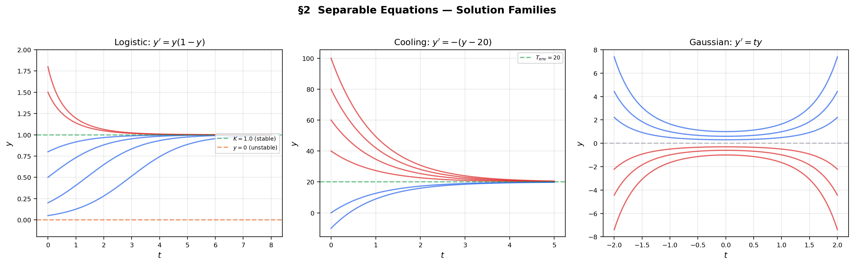
2. Separable Equations
The simplest class of first-order ODEs is the separable equation, where the right-hand side factors as a product of a function of alone and a function of alone. This factorization allows us to move all -terms to one side and all -terms to the other, then integrate each side independently.
📐 Definition 4 (Separable Equation)
An ODE is separable if it can be written as for continuous functions and . The general solution procedure is:
- Separate: .
- Integrate both sides: where and are antiderivatives.
- Solve for if possible, obtaining the solution in explicit form .
📝 Example 2 (Logistic equation)
The logistic equation is separable with and . Partial fractions and integration give the logistic curve
which appears as the sigmoid activation function in ML when , . The solution interpolates between the unstable equilibrium and the stable equilibrium , approaching the carrying capacity from any positive initial condition.
📝 Example 3 (Newton's law of cooling)
The equation models a body at temperature cooling toward ambient temperature . This is separable: . Integrating gives — an exponential decay toward equilibrium.
💡 Remark 2 (Equilibrium solutions and singular points)
When , the constant function is an equilibrium solution (the direction field is horizontal along ). Division by during separation is only valid away from these equilibria. The equilibria of the logistic equation are (unstable) and (stable) — solutions approach from any positive initial condition.
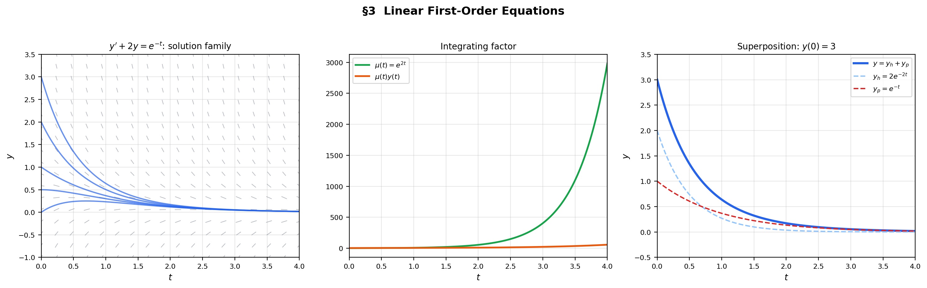
3. Linear First-Order Equations
A linear first-order ODE is not separable (unless ), but it has a systematic solution method: multiply both sides by the integrating factor , which converts the left side into an exact derivative via the product rule.
📐 Definition 5 (Linear First-Order ODE)
An ODE is linear of first order if it has the form
where and are continuous functions on an interval . The equation is homogeneous if and inhomogeneous otherwise.
🔷 Theorem 1 (General Solution of Linear First-Order ODEs)
If and are continuous on an interval containing , then the IVP , has the unique solution
where . In particular, the solution exists on all of — there is no finite-time blow-up for linear equations.
Proof.
Multiply by . The left side becomes by the product rule (Topic 5, Theorem 3): . So
Integrate from to :
Since , solve for :
Uniqueness follows from the Picard-Lindelöf theorem (Theorem 3 below) since is Lipschitz in with .
📝 Example 4 (First-order linear decay with forcing)
Consider , . The integrating factor is . Multiplying: . Integrating: , so . From : . The solution is — the forced response plus a transient that decays faster.
💡 Remark 3 (Linear equations always have global solutions)
Theorem 1 guarantees that the solution exists on the entire interval where and are continuous. This is a stronger result than the general Picard-Lindelöf theorem, which only guarantees local existence. The linearity of the equation prevents finite-time blow-up — the growth rate of is at most exponential, never faster. This global existence result breaks down for nonlinear equations (see Section 7).
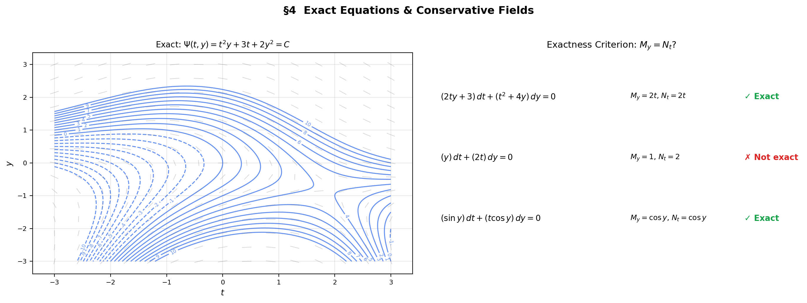
4. Exact Equations & Connection to Conservative Fields
An exact equation is one where the left side is the total differential of some potential function : . The solution curves are the level sets — exactly the conservative field structure from Line Integrals & Conservative Fields.
📐 Definition 6 (Exact Equation)
The equation is exact on a simply connected region if there exists a function with and . The function is the potential function, and solutions are the level curves .
🔷 Theorem 2 (Exactness Criterion)
Let and have continuous first partial derivatives on a simply connected open set . Then is exact if and only if
on . This is the ODE analog of the conservative field criterion from Line Integrals & Conservative Fields (Theorem 4).
📝 Example 5 (An exact equation)
Consider . Check: . So . Then . Solution: .
📝 Example 6 (Integrating factors for non-exact equations)
Consider . Check: . Not exact. Try an integrating factor : we need to depend only on . It does: . Multiplying: . Now — exact. Potential: . Solution: .
💡 Remark 4 (The exact equation ↔ conservative field dictionary)
Exact equations and conservative fields are the same mathematics in different notation. The dictionary:
| ODE | Vector calculus |
|---|---|
| Field with | |
| Exactness: | Irrotational: |
| Solution: | Flow along level curves of the potential |
The simply connected domain requirement (Topic 15, Definition 5) ensures there are no topological obstructions.
5. The Picard-Lindelöf Theorem — Existence and Uniqueness
We now turn to the deepest question in ODE theory: when does an IVP have a solution, and is it unique? The Picard-Lindelöf theorem answers: if is continuous and Lipschitz in , then the IVP , has a unique local solution. The proof uses the contraction mapping principle from Inverse & Implicit Function Theorems (§8) — the same technique that proved the Inverse Function Theorem, now applied in a function space.
📐 Definition 7 (Lipschitz Condition)
A function (with ) satisfies a Lipschitz condition in on if there exists a constant such that
for all . The constant is the Lipschitz constant. If is in and on , then is Lipschitz with constant (by the Mean Value Theorem).
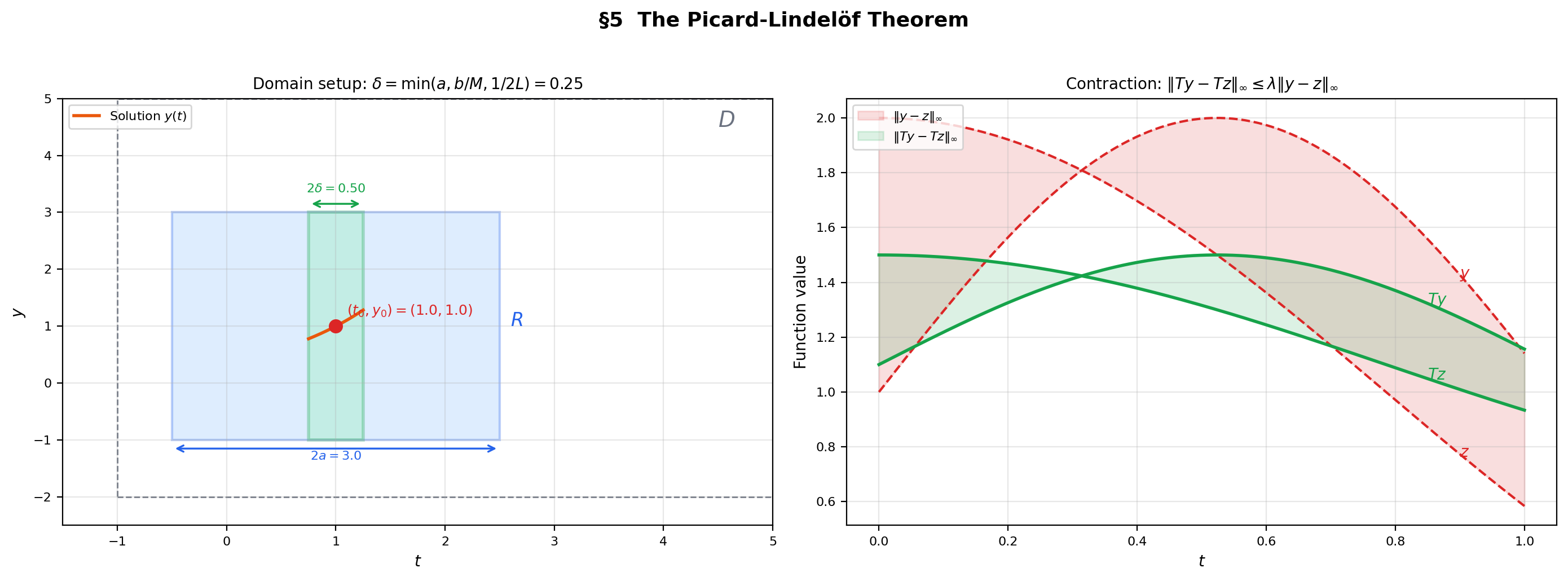
🔷 Theorem 3 (The Picard-Lindelöf Theorem)
Let be continuous on an open set and satisfy a Lipschitz condition in on with Lipschitz constant . Let . Then there exists such that the IVP
has a unique solution .
💡 Remark 5 (Integral formulation)
The IVP , is equivalent to the integral equation
This reformulation is crucial: it converts a differential equation (involving derivatives) into an integral equation (involving only continuous functions and Riemann integration). The Picard iteration is defined in integral form, avoiding the need to differentiate the iterates.
💡 Remark 6 (The Picard-Lindelöf theorem and the IFT — same proof, different spaces)
The structure of the proof is identical to the IFT proof (Topic 12, §8). Define an operator , show it maps a closed set into itself, show it is a contraction, and invoke completeness. The only difference is the space: the IFT works in , while Picard-Lindelöf works in . The reader who followed the IFT proof already knows the playbook.
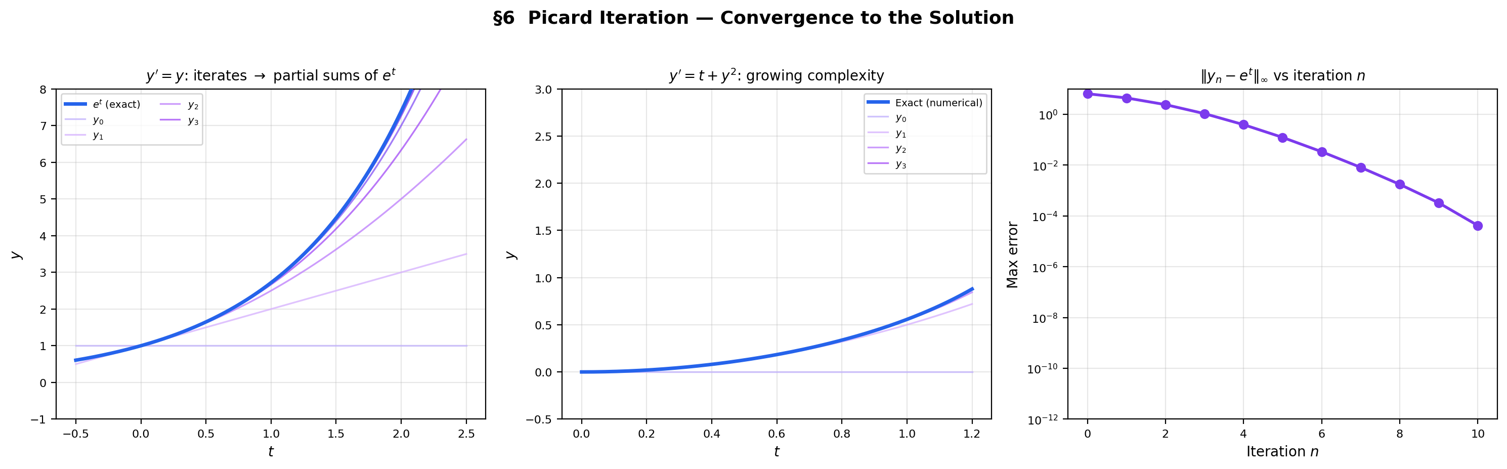
6. Picard Iteration — The Constructive Proof
The Picard-Lindelöf theorem is not merely an existence result — the proof is an algorithm. The Picard iterates
converge uniformly to the unique solution. Each iterate refines the previous approximation, and the Lipschitz condition ensures the refinements shrink geometrically — exactly the contraction mapping mechanism.
📐 Definition 8 (Picard Iteration)
The Picard iterates for the IVP , are defined recursively:
Proof.
We give the full proof via the contraction mapping principle.
Setup. Choose a closed rectangle . Let (which exists since is continuous on the compact set ). Set . Let with the sup-norm , and let . The set is closed in the complete metric space .
Step 1 — maps into . Define the Picard operator by
For :
So .
Step 2 — is a contraction (for small ). For :
If we further require , then . So is a contraction with factor .
Step 3 — Fixed point. The space is a closed subset of a complete metric space, hence complete. By the contraction mapping theorem (Topic 12, Theorem 6), has a unique fixed point :
This is the unique solution to the IVP on .
Step 4 — Convergence of Picard iterates. The contraction mapping theorem also guarantees that uniformly:
The convergence is geometric with rate .
📝 Example 7 (Picard iteration for y' = y, y(0) = 1)
Starting from :
The pattern is — the partial sums of . The Picard iterates converge to the Taylor series of the exact solution .
📝 Example 8 (Picard iteration for y' = t + y², y(0) = 0)
Starting from :
The iterates grow in complexity — no closed-form solution exists for this Riccati equation, but the Picard iterates provide a convergent sequence of polynomial approximations.
7. Maximal Intervals & Blow-Up — When Solutions End
The Picard-Lindelöf theorem guarantees local existence — a solution on some interval . Can the solution always be extended? The maximal interval of existence is the largest interval on which the solution exists. If this interval is bounded, the solution must blow up (escape to infinity) at the boundary.
🔷 Proposition 1 (Extension Theorem)
If is a solution on and exists and lies in , then can be extended past . Equivalently, if cannot be extended past , then either as or approaches the boundary of .
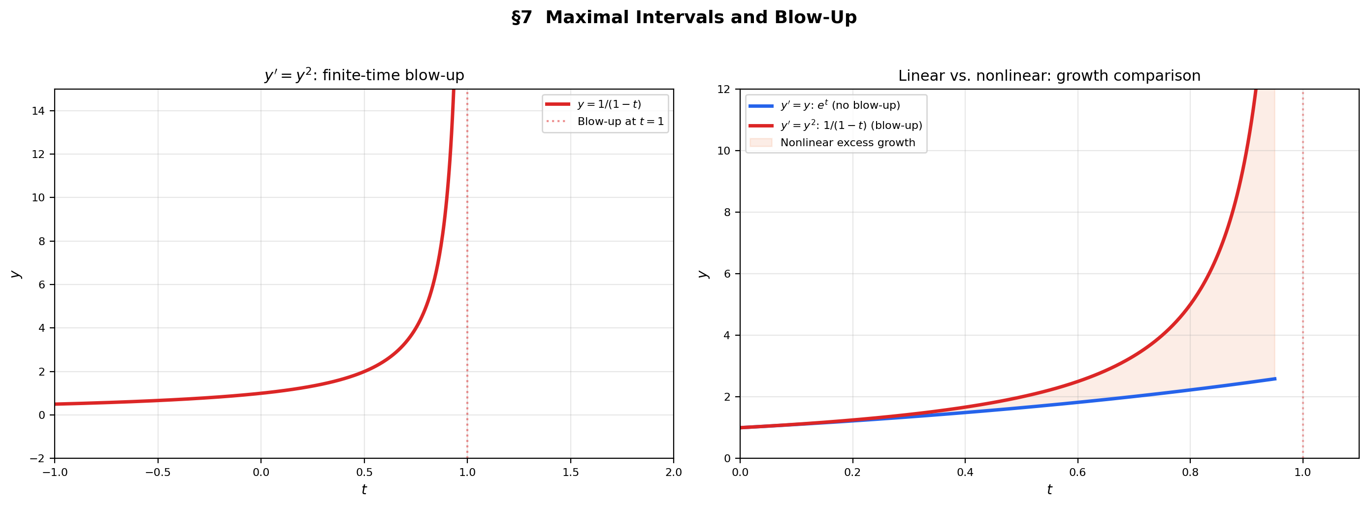
📝 Example 9 (Finite-time blow-up)
Consider , . This is separable: , so . The solution blows up at : as . The maximal interval of existence is , not .
The nonlinearity amplifies growth faster than exponential, causing the solution to reach infinity in finite time. Compare with the linear equation , whose solution grows but never blows up.
💡 Remark 7 (Linear equations never blow up)
Theorem 1 guarantees that solutions to linear equations exist on the entire interval where and are continuous. This is because linear growth prevents finite-time blow-up by Gronwall’s inequality. Nonlinear equations (, , ) can violate this bound and reach infinity in finite time.
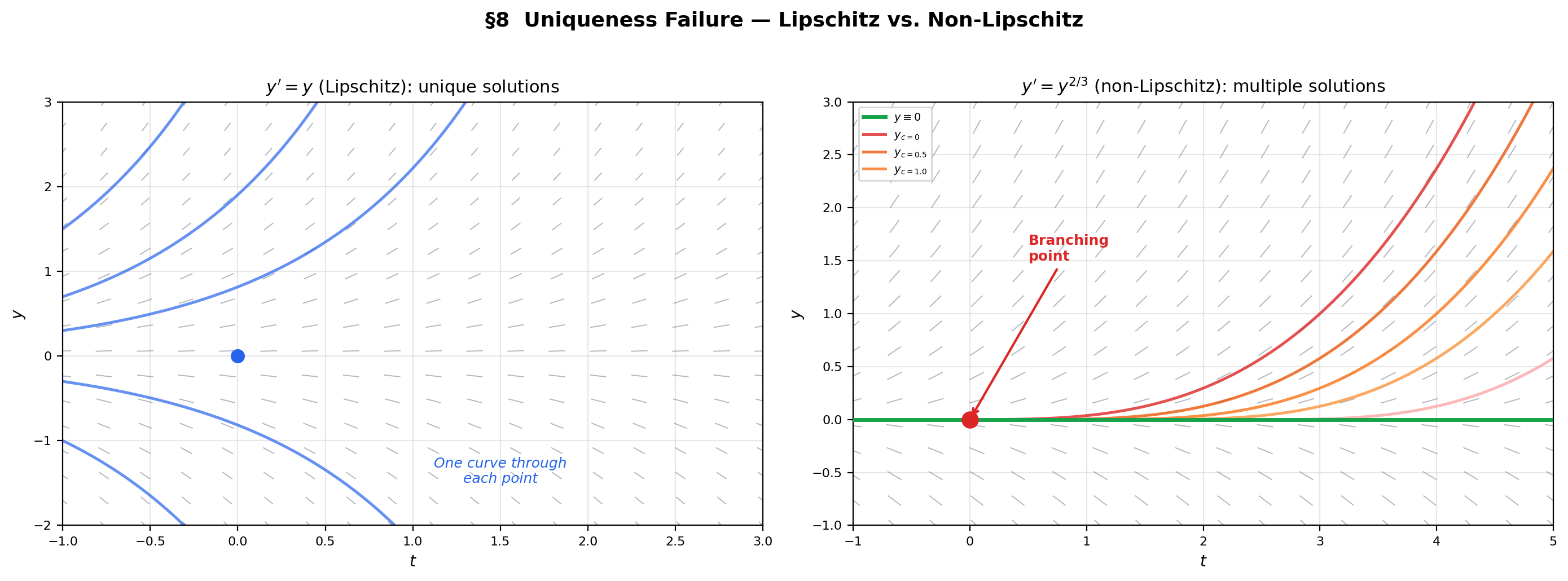
8. Uniqueness Failure — The Peano Theorem and Non-Lipschitz ODEs
What happens without the Lipschitz condition? The Peano existence theorem guarantees that existence requires only continuity of — no Lipschitz condition needed. But uniqueness fails without Lipschitz continuity: multiple solutions can pass through the same initial point, leading to branching trajectories.
🔷 Theorem 4 (Peano Existence Theorem)
If is continuous on an open set containing , then the IVP , has at least one local solution. (No Lipschitz condition required.) The proof uses the Arzelà-Ascoli theorem (compactness in function spaces) rather than contraction mapping.
📝 Example 10 (Uniqueness failure — y' = y^{2/3})
Consider , . The function is continuous but not Lipschitz at (the derivative as ).
Two solutions through :
- (the trivial solution).
- (verified: ).
In fact, for any , the function
is also a solution — there are infinitely many solutions through the origin.
💡 Remark 8 (Why Lipschitz is the right condition)
The Lipschitz condition prevents the right-hand side from changing “too fast” as varies. When is not Lipschitz (as in near ), the direction field near the initial point is too “flat” — nearby solutions cannot distinguish themselves, and multiple integral curves can merge or branch at the non-Lipschitz point. The Lipschitz condition is the minimal regularity that prevents this pathology.
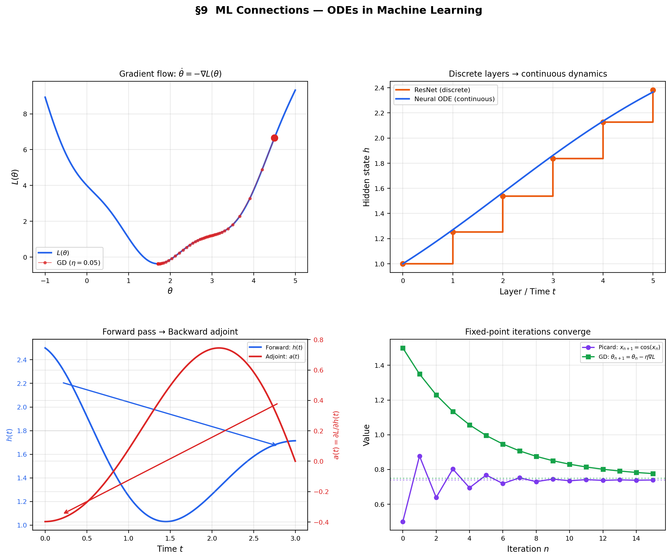
9. ML Connections — Gradient Flow, Neural ODEs, and the Adjoint Method
ODEs are not just classical analysis — they are the mathematical backbone of several central ideas in modern machine learning. Gradient descent is a discretized ODE. Neural ODEs replace discrete layers with continuous dynamics. The Picard iteration is a fixed-point computation analogous to training.
9.1 Gradient flow as an ODE
Gradient descent is the Euler discretization (step size ) of the gradient flow ODE
When is Lipschitz (with constant ), the Picard-Lindelöf theorem guarantees the gradient flow has a unique trajectory from any initial . Convergence of the continuous flow to a critical point () is analyzed by treating as a Lyapunov function:
The loss decreases monotonically along the flow — the continuous-time version of the “gradient descent decreases the loss” guarantee. The learning rate controls how well the discrete steps approximate the continuous trajectory.
→ Gradient Descent → formalML
9.2 Neural ODEs
Chen et al. (2018) observed that a residual network (where indexes layers, not time) is the Euler discretization of . Replacing discrete layers with the continuous ODE yields a neural ODE: the forward pass solves the IVP , using a black-box ODE solver (Runge-Kutta, adaptive stepping — see Numerical Methods for ODEs).
The Picard-Lindelöf theorem guarantees the forward pass has a unique solution when is Lipschitz in , which holds when the network weights are bounded. Memory cost is regardless of depth (the ODE solver stores only the current state), whereas a residual network with layers incurs memory cost.
9.3 The adjoint method
Backpropagation through a neural ODE cannot store intermediate activations (there are infinitely many “layers”). Instead, the adjoint method computes gradients by solving a second ODE backward in time. Define the adjoint . Then satisfies the adjoint ODE
integrated backward from . The gradient with respect to parameters is
This is another first-order ODE — and its existence is guaranteed by Picard-Lindelöf under the same Lipschitz conditions.
9.4 Picard iteration as a training analog
The Picard iteration converges to a fixed point of the operator . Training a neural network is also a fixed-point iteration — it converges to a fixed point of the gradient descent operator. Deep equilibrium models (DEQs, Bai et al. 2019) make this analogy explicit: the forward pass finds a fixed point by iterating until convergence, and backpropagation through the fixed point uses the Implicit Function Theorem to compute .
→ Smooth Manifolds → formalML → Measure-Theoretic Probability → formalML
10. Computational Notes
- Direction field visualization: Compute on a grid and draw line segments with slope at each gridpoint. Grid density should be at least 20×20 for visual clarity. Normalize segment lengths by to keep the display uniform.
- Numerical solution:
scipy.integrate.solve_ivpsolves IVPs with adaptive Runge-Kutta methods (default: RK45). For stiff equations, usemethod='Radau'or'BDF'. The Picard iteration converges in theory, but is impractical for computation — the integrals become intractable after a few iterations for most equations. - Blow-up detection: Adaptive solvers detect blow-up when the step size shrinks below machine epsilon. Setting
max_stepand monitoring can provide early warning. - Lipschitz constant estimation: For with bounded , estimate numerically: , computed on a grid via the Mean Value Theorem.
11. Closing Reflection — The ODE Track Begins
This is the first of four topics in the Ordinary Differential Equations track. The track progresses from first-order scalar equations (this topic) to systems and the matrix exponential (Linear Systems & Matrix Exponential), to qualitative analysis of equilibria and stability (Stability & Dynamical Systems), and finally to numerical methods (Numerical Methods for ODEs). The thread connecting them all is the interplay between existence (does a solution exist?), structure (what does the solution look like?), and computation (how do we find it?).
Connections & Further Reading
Prerequisites — topics you need first
Inverse & Implicit Function Theorems
The contraction mapping principle from Topic 12 (§8) is the proof engine of the Picard-Lindelöf theorem. The pattern is identical — define an iteration operator T, prove it is a contraction under the sup-norm, invoke completeness to get a fixed point — but applied in the function space C([t₀ − δ, t₀ + δ]) instead of ℝⁿ. The reader who understood the IFT proof already knows the script.
The Derivative & Chain Rule
An ODE y' = f(t, y) is an equation involving the derivative — the foundational object from Topic 5. The product rule drives the integrating factor method, implicit differentiation verifies solutions obtained by separation, and the chain rule underpins the conversion between implicit and explicit solution forms.
Line Integrals & Conservative Fields
Exact differential equations M dt + N dy = 0 with M_y = N_t are the ODE analog of conservative vector fields from Topic 15. The exactness criterion is identical, and the solution method (finding a potential function) is the same. The integrating factor technique converts non-exact equations into exact ones, paralleling the search for a potential function.
The Riemann Integral & FTC
The Picard iteration y_{n+1}(t) = y₀ + ∫f(s, yₙ(s))ds involves Riemann integration at every step. The integral formulation of the IVP — y(t) = y₀ + ∫f(s, y(s))ds — is the starting point for both the existence proof and numerical methods.
Completeness & Compactness
The Picard-Lindelöf proof requires the completeness of the function space (C([a,b]), ‖·‖∞). A Cauchy sequence of continuous functions converges to a continuous function under the sup-norm — the same completeness property from Topic 3 applied in an infinite-dimensional setting.
Mean Value Theorem & Taylor Expansion
The Lipschitz condition |f(t, y₁) − f(t, y₂)| ≤ L|y₁ − y₂| is implied by a bound on the partial derivative: if |∂f/∂y| ≤ L on the domain, then the Mean Value Theorem gives the Lipschitz estimate. Taylor expansion is used to analyze local behavior of solutions near equilibria.
Where this leads — next in formalCalculus
Linear Systems & Matrix Exponential
Systems y' = Ay generalize scalar linear equations; the matrix exponential e^(At) extends the scalar solution e^(at) to vector-valued trajectories.
Numerical Methods for ODEs
Euler's method is the simplest discretization; RK4 and adaptive methods are the workhorses. The Picard iteration is impractical for computation — numerical methods take over.
Stability & Dynamical Systems
Phase portraits and Lyapunov stability classify the long-time behavior near equilibria — existence and uniqueness from this topic ensure trajectories never cross, enabling the qualitative theory.
Metric Spaces & Topology
The Banach Contraction Mapping Theorem is proved in full, giving the abstract result that powers the Picard-Lindelöf argument here and the Inverse Function Theorem from Topic 12.
On to formalStatistics — where this calculus powers inference
On to formalML — where this calculus powers ML
Gradient Descent
Gradient descent is the Euler discretization of gradient flow θ̇ = −∇L(θ), a first-order ODE. The Picard-Lindelöf theorem guarantees the existence and uniqueness of the gradient flow trajectory when ∇L is Lipschitz, the smoothness assumption underlying most convergence proofs. The learning rate η is the Euler step size, and a smaller η yields a better approximation of the continuous trajectory.
Smooth Manifolds
A vector field X on a smooth manifold M defines a first-order ODE: the integral curves of X are the solutions. The existence and uniqueness theorem guarantees local integral curves exist, and the flow map Φ_t: M → M is a local diffeomorphism. This is the ODE-theoretic foundation of dynamical systems on manifolds.
Measure Theoretic Probability
Stochastic differential equations dX_t = f(X_t)dt + σ(X_t)dW_t extend deterministic ODEs by adding Brownian noise. Itô's existence theorem is the stochastic analog of Picard-Lindelöf, using the same Lipschitz condition and contraction argument in a space of stochastic processes.
References
- book Arnold (1992). Ordinary Differential Equations Chapters 1–4 develop the geometric viewpoint: ODEs as vector fields, integral curves as trajectories, the phase plane. The primary reference for our geometric-first approach and the direction field visualizations
- book Teschl (2012). Ordinary Differential Equations Chapters 1–2 provide a rigorous treatment of existence and uniqueness via the contraction mapping principle. Available free online. Our model for the Picard-Lindelöf proof structure
- book Rudin (1976). Principles of Mathematical Analysis Chapter 9 (Theorem 9.12) proves the Picard-Lindelöf theorem as a contraction mapping application, connecting to the IFT proof in the same chapter. Useful for the condensed proof style
- book Boyce & DiPrima (2012). Elementary Differential Equations and Boundary Value Problems Chapters 2–3 provide the standard undergraduate treatment of first-order methods (separable, linear, exact) with extensive examples. Reference for the computational sections
- paper Chen, Rubanova, Bettencourt & Duvenaud (2018). “Neural Ordinary Differential Equations” The foundational neural ODE paper — replaces discrete residual layers with continuous dynamics, uses the adjoint method for backpropagation. The primary ML connection for this topic
- paper Massaroli, Poli, Park, Yamashita & Asama (2020). “Dissecting Neural ODEs” A comprehensive analysis of neural ODE architectures, training dynamics, and expressiveness. Complements the Chen et al. paper with practical insights
- paper Santurkar, Tsipras, Ilyas & Madry (2018). “How Does Batch Normalization Help Optimization?” Shows that batch normalization smooths the loss landscape, making ∇L Lipschitz — exactly the condition needed for Picard-Lindelöf to guarantee gradient flow solutions