The Derivative & Chain Rule
Rates of change as limits of difference quotients — the tangent line as the best linear approximation, differentiation rules from first principles, and the chain rule that makes backpropagation possible
Abstract. The derivative of f at a is the limit f'(a) = lim_{h→0} [f(a+h) - f(a)] / h — the instantaneous rate of change, the slope of the tangent line, and the best linear approximation to f near a, all in one definition. Geometrically, the derivative is what you get when secant lines through (a, f(a)) and (a+h, f(a+h)) converge as h → 0: the limiting slope is f'(a), and the limiting line is the tangent. This limit need not exist — |x| is continuous at 0 but has no derivative there because the left and right secant slopes disagree, and the Weierstrass function is continuous everywhere but differentiable nowhere. When the derivative does exist, differentiability implies continuity (but not the converse), and differentiation obeys algebraic rules derived directly from the limit definition: the sum rule, the product rule (Leibniz rule), the quotient rule, and — most importantly — the chain rule (f ∘ g)'(a) = f'(g(a)) · g'(a). The chain rule says that the derivative of a composition is the product of the derivatives along the chain. This is not a coincidence — it reflects the fact that the derivative at each point is a linear map, and composing linear maps means multiplying them. In machine learning, the chain rule is used in backpropagation: given a loss L = L(f(g(h(x)))), the gradient ∂L/∂x is computed by multiplying local derivatives and backpropagating them through the computation graph, which is exactly the chain rule applied layer by layer. Automatic differentiation (reverse mode = backprop, forward mode = tangent propagation) mechanizes this process, and every gradient-based optimizer — SGD, Adam, RMSProp — depends on the chain rule to compute the gradients it needs.
Overview & Motivation
Every time you train a neural network, you watch a loss curve drop. The optimizer adjusts each parameter by a small step — but in which direction, and how far? The answer is the derivative: tells you the rate at which the loss changes with respect to , and that rate determines both the direction (the sign of ) and the magnitude (||) of the update.
But a modern network doesn’t have one parameter — it has millions, composed in layers. The input passes through , then , then , and so on. To compute for a parameter buried in , we need to differentiate through the entire chain of compositions. This is the chain rule: the derivative of a composition is the product of the derivatives at each stage. And backpropagation — the algorithm that makes deep learning computationally feasible — is simply the chain rule applied systematically to a computation graph.
This topic makes both the derivative and the chain rule precise. We start with the geometric picture — secant lines rotating into the tangent — define the derivative as a limit, derive the differentiation rules from first principles, and prove the chain rule using the linear approximation characterization. By the end, you’ll see exactly why backpropagation works and what “taking the gradient” means at the level of individual arithmetic operations.
Prerequisites: We use the limit definition from Sequences, Limits & Convergence — specifically, the algebra of limits (Theorem 3) — and the ε-δ framework from Epsilon-Delta & Continuity for the function limit that defines .
The Derivative as a Limit
Two points, one slope
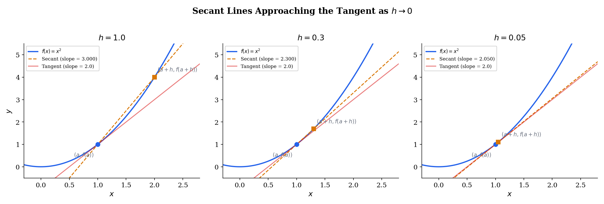
Consider a function and two points on its graph: and , where . The straight line through these two points is a secant line, and its slope is the difference quotient:
This ratio measures the average rate of change of between and . When is large, the secant line is a crude summary — it ignores everything the function does between the two points. But as shrinks toward , the secant line pivots around and settles into a unique position: the tangent line. The slope of that tangent is the instantaneous rate of change — the derivative.
📐 Definition 1 (The Derivative)
Let be defined on an open interval containing . The derivative of at is
provided this limit exists. Equivalently, using the ε-δ framework from Epsilon-Delta & Continuity: for every , there exists such that
When this limit exists, we say is differentiable at . The function , defined at every point where the limit exists, is the derivative function of .
The notation is Lagrange’s. We also write (Leibniz) or (Euler/operator notation). The Leibniz notation is suggestive — it looks like a ratio of infinitesimals — and in practice we often manipulate it as if it were one. But the definition above is what makes it rigorous: is a single number, the limit of a ratio, not a ratio of limits.
📐 Definition 2 (Left and Right Derivatives)
The left derivative and right derivative of at are
The derivative exists if and only if both one-sided derivatives exist and .
This connects directly to one-sided limits from Epsilon-Delta & Continuity — the derivative is defined by a function limit as , and that limit exists if and only if both one-sided limits agree.
📝 Example 1 (Derivative of f(x) = x² at a = 3)
We compute directly from the definition:
Every step is algebra followed by a limit. The cancellation of in the numerator and denominator is the key move — it removes the indeterminate form and leaves a polynomial in that we can evaluate at .
📝 Example 2 (Derivative of f(x) = √x at a > 0)
For at :
The direct approach gives , so we rationalize — multiply numerator and denominator by the conjugate :
As , this converges to . So , which is defined for — the domain of the derivative is smaller than the domain of (which includes ). At , the difference quotient , so is not differentiable there (vertical tangent).
Try dragging the slider toward zero in the explorer below — watch how the secant line (amber) rotates into the tangent line (red dashed), and how the secant slope converges to .
The Derivative as Linear Approximation
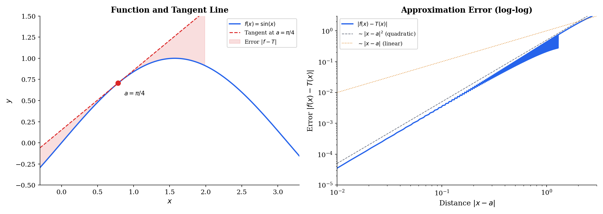
The tangent line is more than a geometric artifact — it is the best linear approximation to near . The tangent line at is
and the quality of this approximation is measured by the error . The defining property of the derivative is that this error vanishes faster than the distance from :
🔷 Proposition 1 (Derivative as Best Linear Approximation)
is differentiable at with derivative if and only if there exists a number such that
where . The number is unique and equals . The remainder is said to be “little-o of ”, written .
This characterization is the conceptual bridge to multivariable calculus. In one dimension, the “linear map” is just multiplication by a scalar. But the same definition works in : the derivative of at is the linear map such that . That linear map is represented by the Jacobian matrix — and the chain rule becomes matrix multiplication. The single-variable case is the prototype.
💡 Remark 1 (Linear maps preview)
In one dimension, a linear map is multiplication by a scalar: . The derivative is that scalar. In , the derivative at will be a matrix (the Jacobian ), and “multiplication by a scalar” becomes “multiplication by a matrix.” The single-variable derivative is the case of the Jacobian.
Explore the tangent line below — drag the point along the curve and notice how the error (right panel) decays quadratically near , confirming that the tangent is truly the best linear approximation.
Differentiability and Continuity
A natural question: if is differentiable at , must it be continuous there? And conversely: if is continuous at , must it be differentiable? The answers are “yes” and “no,” respectively — and both answers are important.
🔷 Theorem 1 (Differentiability Implies Continuity)
If is differentiable at , then is continuous at .
Proof.
We need to show that , which is continuity at (Epsilon-Delta & Continuity, Definition 5). Write
As , the first factor converges to (by differentiability) and the second factor converges to . By the algebra of limits (Sequences, Limits & Convergence, Theorem 3), the product converges to . So , which means . ∎
💡 Remark 2 (The converse is false)
Continuity does not imply differentiability. The function is continuous everywhere — including at — but is not differentiable at . This is not a pathological edge case: every ReLU unit in a neural network has a corner at with the same non-differentiability as . In practice, ML frameworks define the “derivative” at the kink by convention (typically or ), which works because the set of inputs landing exactly on the kink has measure zero.
📝 Example 3 (f(x) = |x| is not differentiable at 0)
The left derivative at :
The right derivative at :
Since , the derivative does not exist. Geometrically, the graph of has a corner at — there is no single tangent line, because the secant from the left settles on slope while the secant from the right settles on slope .
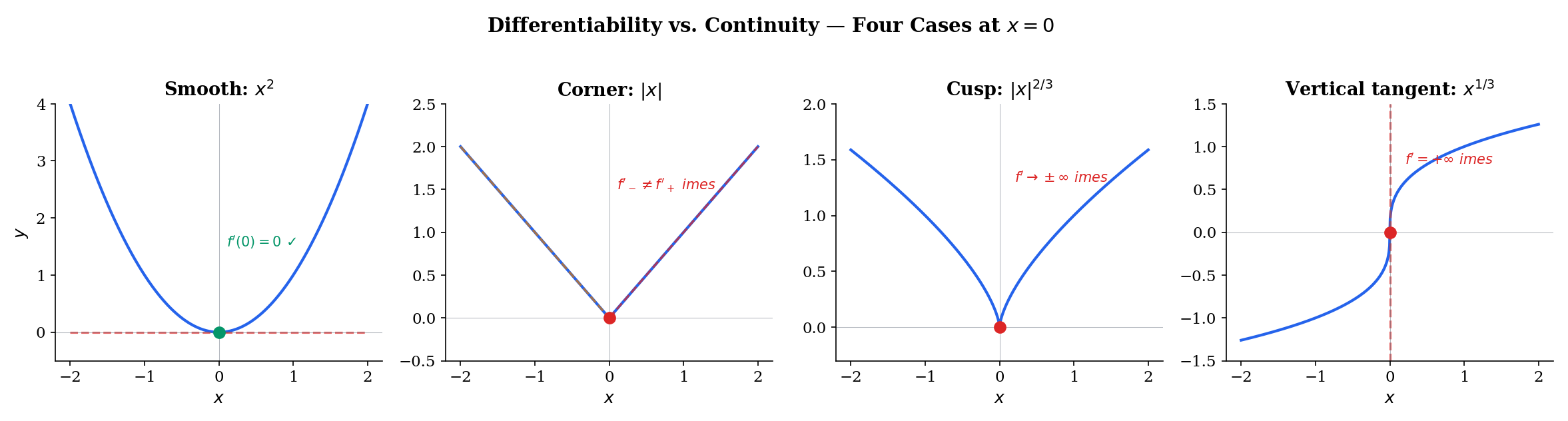
Use the tabs below to compare smooth, corner, cusp, and Weierstrass-type non-differentiability. Drag the slider toward zero and watch whether the left and right secant slopes agree.
f(x) = x² is differentiable everywhere. Both left and right difference quotients converge to f'(0) = 0.
Differentiation Rules
Computing derivatives from the limit definition every time would be tedious. Fortunately, the limit definition yields general rules that handle sums, products, quotients, and powers. We derive each rule from the definition — no shortcuts, no “it can be shown.”
🔷 Theorem 2 (Sum Rule)
If and are differentiable at , then is differentiable at and
Proof.
Taking the limit as and applying the sum rule for limits (Sequences, Limits & Convergence, Theorem 3), we get . ∎
🔷 Theorem 3 (Constant Multiple Rule)
If is differentiable at and , then .
The proof is identical — factor out of the difference quotient and use the constant multiple rule for limits.
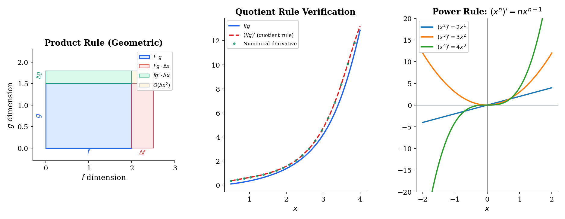
🔷 Theorem 4 (Product Rule (Leibniz Rule))
If and are differentiable at , then is differentiable at and
Proof.
The key is the add-and-subtract trick. Write
Factor:
Divide by :
As : the first term converges to (using Theorem 1: is differentiable hence continuous, so ), and the second term converges to . By the algebra of limits, the sum converges to . ∎
🔷 Theorem 5 (Quotient Rule)
If and are differentiable at and , then is differentiable at and
Proof.
Write the difference quotient:
Add and subtract in the numerator:
Split the fraction and take the limit. The numerator converges to . The denominator converges to (since is continuous at by Theorem 1, so , and ensures the limit is well-defined). ∎
📝 Example 4 (The power rule via the binomial theorem)
For with a positive integer:
As , every term with vanishes (it contains to a positive power), leaving only the term:
This is the power rule: .
The Chain Rule
The chain rule is the most important theorem in this topic — and arguably the most consequential single result for machine learning. It tells us how to differentiate a composition , and the answer is beautifully simple: the derivative of the composition is the product of the derivatives.
Geometric intuition
Think of as a function that stretches the input near by a factor of , and as a function that stretches the input near by a factor of . When we compose them — first stretches, then stretches — the total stretching is the product: .
This is exactly what “the derivative of a composition is the product of the derivatives” means geometrically: each function contributes its own local stretching factor, and stretching factors multiply.
🔷 Theorem 6 (The Chain Rule)
If is differentiable at and is differentiable at , then is differentiable at and
Proof.
We use the linear approximation characterization (Proposition 1). Since is differentiable at , we can write
where as (and we define ).
The subtle point: A naive proof would divide by and recombine, but this fails when for (which can happen — for example, with ). The linear approximation approach avoids division entirely.
Set . Then
Subtract and divide by :
As : the factor by differentiability of , and (by continuity of , which follows from differentiability via Theorem 1), so . By the algebra of limits:
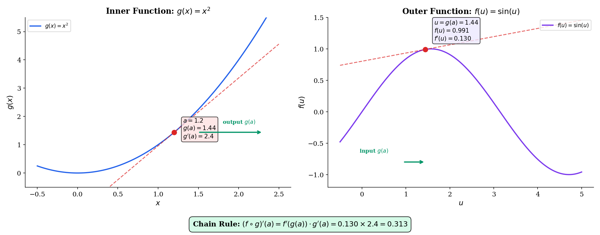
📝 Example 5 (Chain rule: d/dx sin(x²))
Let and , so .
- Inner derivative:
- Outer derivative: , evaluated at :
- Chain rule:
At : .
📝 Example 6 (Three-layer chain rule: d/dx e^{sin(x²)})
This is a composition of three functions: , , . The chain rule applies iteratively:
Three derivatives, multiplied in order from outermost to innermost. This is a three-layer “network” — the chain rule applies at each layer. In a neural network with layers, we would multiply local derivatives.
💡 Remark 3 (The chain rule as composition of linear maps)
Each derivative is a linear map (multiplication by ). The chain rule says: the derivative of a composition is the composition of the derivatives. In one dimension, composing two linear maps means multiplying two scalars: .
In , “multiplication” becomes matrix multiplication:
where and are Jacobian matrices. The chain rule is functorial — it respects the compositional structure of functions. This perspective is the starting point for differential geometry, where the derivative is the pushforward map between tangent spaces. (→ formalML: Smooth Manifolds)
Explore the chain rule visually below — the left panel shows the inner function with its tangent, and the right panel shows the outer function with its tangent at . The derivative readout shows the product of local derivatives.
Higher-Order Derivatives
If is itself a function, we can ask: is differentiable? If so, its derivative is the second derivative of .
📐 Definition 3 (Higher-Order Derivatives)
The second derivative of at is , provided is differentiable at . Inductively, the -th derivative is .
Notation: or for the second derivative; or for the -th derivative.
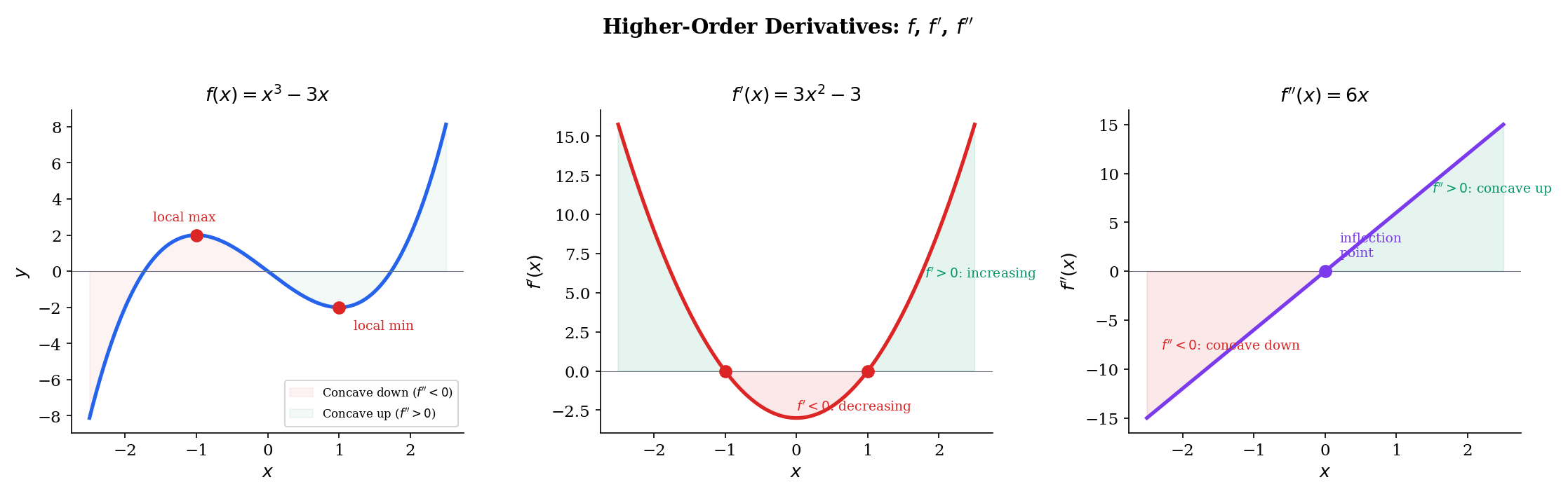
💡 Remark 4 (Concavity and the second derivative)
The sign of determines the concavity of at :
- : is concave up at — the graph curves upward, and the tangent line lies below the graph. This is the 1D condition for a local minimum.
- : is concave down at — the graph curves downward, and the tangent line lies above the graph. This is the 1D condition for a local maximum.
In higher dimensions, the second derivative becomes the Hessian matrix , and “concave up” becomes “positive definite” — the multi-dimensional criterion for a local minimum. This is the foundation of Newton’s method and second-order optimization. (The Hessian & Second-Order Analysis (coming soon))
Non-Differentiable Functions
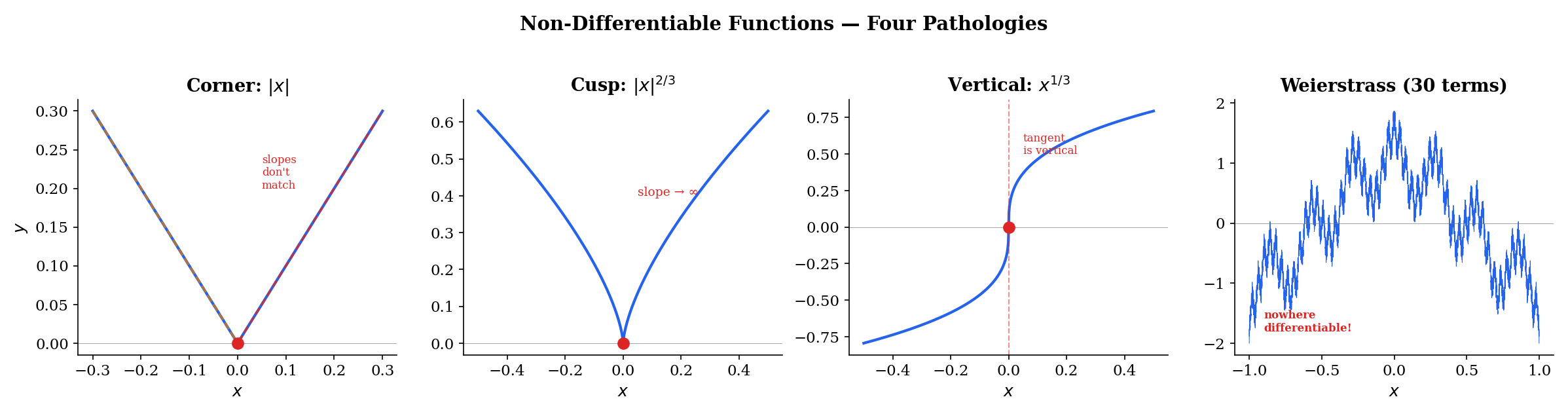
Differentiability is a strong condition — stronger than continuity. There are several ways it can fail:
1. Corners. The function is continuous everywhere but has a corner at where the left and right derivatives disagree ( and ). This is exactly the non-differentiability of ReLU at zero.
2. Cusps. The function is continuous at but the difference quotient as . The curve comes to a sharp point where the “tangent line” would be vertical — but vertical lines have undefined slope.
3. Vertical tangents. The function at has a difference quotient . The tangent exists visually (it’s the -axis), but its slope is infinite, so the derivative does not exist as a real number.
4. Everywhere non-differentiable. The Weierstrass function
is continuous everywhere (by the Weierstrass M-test, which we proved in Uniform Convergence) but differentiable nowhere. The partial sums are smooth, but each additional term adds higher-frequency oscillations. No matter how far you zoom in, the graph never smooths out — there is no tangent line at any point.
💡 Remark 5 (Non-differentiability in ML)
ReLU has a corner at — the same non-differentiability as shifted. In practice, ML frameworks assign a conventional “derivative” at the kink ( or ), and this works because:
- The set of inputs landing exactly on the kink has Lebesgue measure zero — almost every input avoids it. (Sigma-Algebras & Measures (coming soon))
- The difference quotient from either side is well-defined (it’s or ), so the “gradient” used in practice is the one-sided derivative — which is fine for optimization.
The Weierstrass function shows that pathology can be extreme — continuous everywhere, differentiable nowhere — but such functions don’t arise as loss landscapes in practice. Real neural network losses are piecewise smooth (smooth between the ReLU kinks), and that’s smooth enough for gradient descent.
Connections to Statistics
The derivative is the foundation of every optimization-based estimator in statistics. The score function, Fisher information, Cramér–Rao bound, and the asymptotic theory of maximum likelihood are all built from first and second derivatives of the log-likelihood.
The score and the MLE
The score function is literally the derivative of the log-likelihood; Fisher information is the second derivative. The MLE solves — a derivative-equals-zero condition — and its asymptotic variance is . See formalStatistics Maximum Likelihood.
Score and Wald tests
The score test statistic and the Wald statistic are both built from first and second derivatives of the log-likelihood. Their asymptotic chi-squared distributions follow from a Taylor expansion of the log-likelihood around . See formalStatistics Likelihood Ratio Tests & Neyman–Pearson.
Delta method and the Cramér–Rao bound
The Cramér–Rao lower bound differentiates under the integral sign — a maneuver justified by dominated-convergence conditions. The delta method for estimators of the form is a first-order Taylor expansion: , giving asymptotic variance . See formalStatistics Point Estimation.
Connections to ML — Backpropagation & Automatic Differentiation
This is where the derivative and chain rule connect directly to modern machine learning practice. Backpropagation is not a separate algorithm — it is the chain rule, applied systematically to a computation graph.
Backpropagation is the chain rule
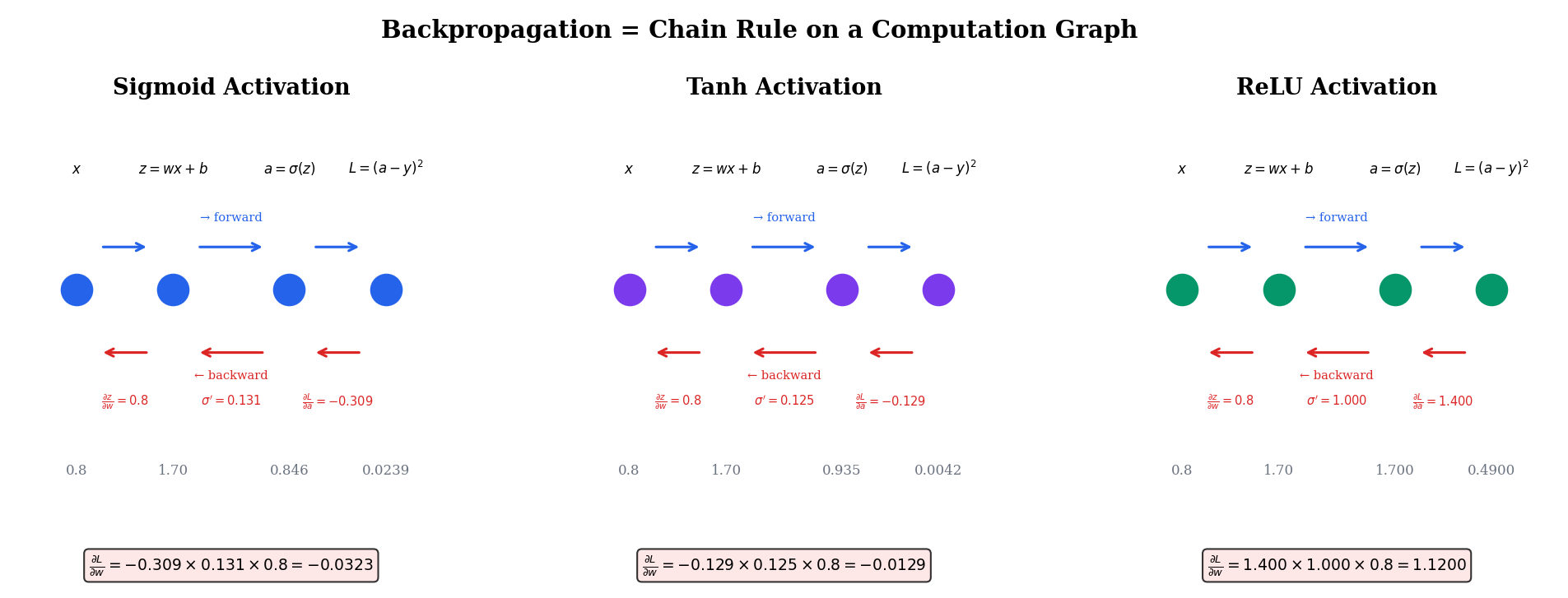
Consider a minimal network: input , weight , bias , activation , target , and loss :
The forward pass computes , then , then — evaluating the composition left to right. The backward pass computes gradients right to left using the chain rule:
Each factor is a local derivative — the derivative of one node with respect to its immediate input. The chain rule says the total derivative is the product of the locals. This is exactly Theorem 6 applied to the composition .
Automatic differentiation
Forward mode (tangent propagation): set and propagate forward: , , . Cost: one forward sweep per input variable.
Reverse mode (backpropagation): set and propagate backward: , , . Cost: one backward sweep for all parameters.
For a network with millions of parameters and a scalar loss, reverse mode wins by a factor of millions — this is why backpropagation, not forward-mode AD, is the standard in deep learning.
Common activation derivatives
| Activation | ||
|---|---|---|
| Sigmoid | ||
| Tanh | ||
| ReLU |
The sigmoid and tanh derivatives both compress toward zero for large — this is the vanishing gradient problem. ReLU avoids it (gradient is for ) at the cost of the non-differentiability at . (→ formalML: Gradient Descent)
Explore the computation graph below — toggle between forward and backward pass to see how values and gradients flow through the network.
Computational Notes
When we don’t have a closed-form derivative, we can approximate numerically using finite differences:
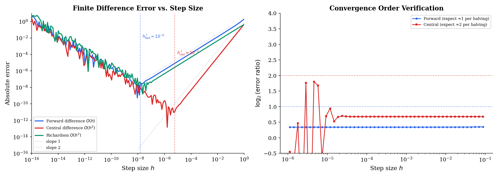
Forward difference: . Truncation error is , but catastrophic cancellation occurs at very small (around for double precision).
Central difference: . The odd-order error terms cancel, giving accuracy — a quadratic improvement over forward differences. Optimal .
Richardson extrapolation: Combine central differences at and to cancel the leading error term: . Each level of extrapolation eliminates one more error term.
The tradeoff: smaller reduces truncation error but increases floating-point cancellation error. There is an optimal that balances both — roughly for a method of order , where for double precision.
Connections & Further Reading
Prerequisites — topics you need first
Sequences, Limits & Convergence
The derivative is defined as a limit. The convergence theory from Topic 1 — the ε-N definition, limit uniqueness, the algebra of limits — provides the rigorous foundation for the difference quotient limit that defines f'(a).
Epsilon-Delta & Continuity
The limit in the derivative definition is a function limit (h → 0), formalized by the ε-δ framework from Topic 2. The proof that differentiability implies continuity uses ε-δ continuity directly.
Where this leads — next in formalCalculus
On to formalStatistics — where this calculus powers inference
Maximum Likelihood
The score function U(θ) = ∂/∂θ log L(θ) is literally the derivative of the log-likelihood; Fisher information I(θ) = -E[∂²/∂θ² log L] is the second derivative. The MLE θ̂ solves U(θ̂) = 0 — a derivative-equals-zero condition.
Likelihood Ratio Tests And Np
The score test statistic U(θ_0)²/I(θ_0) and the Wald statistic (θ̂ - θ_0)²·I(θ̂) are both built from first and second derivatives of the log-likelihood. The asymptotic chi-squared distribution follows from a Taylor expansion around θ_0.
Point Estimation
The Cramér–Rao lower bound differentiates under the integral sign — a maneuver justified by dominated-convergence conditions. The delta method for estimators of the form g(θ̂) is a first-order Taylor expansion: g(θ̂) ≈ g(θ) + g'(θ)(θ̂ - θ).
Central Limit Theorem
Topic 11's MGF-based CLT proof Taylor-expands the MGF to extract the limiting characteristic function; the remainder bound from differentiation theory is the source of the o(1) error. The delta method √n(g(X̄_n) − g(μ)) → N(0, g'(μ)²σ²) is a first-order Taylor expansion requiring g to be differentiable.
Confidence Intervals And Duality
Topic 19's profile likelihood ℓ_P(θ) = sup_ψ ℓ(θ, ψ) is differentiated via the Danskin envelope theorem (§19.7 Rem 15); the implicit-function maneuver pairs with the chain rule developed here to handle the nuisance score equation ψ̂(θ).
Hypothesis Testing
Topic 17 differentiates the power function β(θ) to characterize most-powerful tests (preview §17.4, full treatment Topic 18). The score test statistic U(θ_0) = ∂_θ ℓ(θ_0) is the derivative of the log-likelihood evaluated at the null.
Large Deviations
Topic 12's Chernoff bound optimizes over the tilting parameter t via first-order conditions; the Cramér rate function I(x) = sup_t(tx − log M(t)) is a convex conjugate (Legendre transform) requiring differentiation to evaluate. Taylor expansion enters the Hoeffding lemma's bound for bounded random variables.
Method Of Moments
Topic 15's delta method uses the Jacobian of the moment-to-parameter map (a multivariate chain rule); the M-estimator sandwich variance A⁻¹BA⁻¹^T uses partial derivatives of the estimating function ψ(x; θ) with respect to θ.
Sufficient Statistics
Topic 16's Pitman–Koopman–Darmois proof cross-differentiates the log-factorization in the data argument and the parameter — equality of mixed partial derivatives reveals the separable structure that characterizes exponential families.
On to formalML — where this calculus powers ML
Gradient Descent
Single-variable gradient descent θ_{t+1} = θ_t - η f'(θ_t) is the prototype for all gradient methods. The chain rule enables backpropagation — computing gradients through compositions of functions (network layers) — which is the computational engine of gradient-based optimization.
Shannon Entropy
Derivatives of entropy H(p) = -Σ pᵢ log pᵢ, KL divergence, and cross-entropy loss are central to information-theoretic ML objectives. The derivative d/dp(-p log p) = -log p - 1 connects information content to optimization.
Smooth Manifolds
The single-variable derivative is the 1D prototype for the pushforward map between tangent spaces. Differentiable functions are the morphisms of smooth manifolds — the chain rule becomes functoriality of the tangent functor.
References
- book Abbott (2015). Understanding Analysis Chapter 5 develops the derivative from the limit definition through the Mean Value Theorem — the primary reference for our rigorous-but-accessible approach
- book Rudin (1976). Principles of Mathematical Analysis Chapter 5 on differentiation — the compact, definitive treatment of single-variable derivatives
- book Spivak (2008). Calculus Chapters 9–11 develop differentiation with unusual care for geometric intuition alongside full rigor — exceptional treatment of the chain rule proof
- book Goodfellow, Bengio & Courville (2016). Deep Learning Section 6.5 on back-propagation — the chain rule as the computational engine of deep learning
- paper Baydin, Pearlmutter, Radul & Siskind (2018). “Automatic Differentiation in Machine Learning: a Survey” Comprehensive survey of forward-mode and reverse-mode AD — mechanizing the chain rule for gradient computation