Numerical Methods for ODEs
From Euler's method to adaptive solvers — error analysis, stability regions, stiff systems, and the convergence theory that guarantees discrete approximations track continuous solutions. The computational engine behind neural ODEs.
Abstract. We can prove solutions to y' = f(t,y) exist (Picard-Lindelöf) and analyze their stability (Lyapunov theory) — but how do we actually compute them? Euler's method replaces the derivative with a finite difference: y_{n+1} = y_n + h·f(t_n,y_n). This is first-order accurate — global error grows as O(h). Runge-Kutta methods evaluate f at intermediate points to achieve higher accuracy: the classical RK4 is O(h⁴). But accuracy is not enough. For stiff systems — where the Jacobian eigenvalues span many orders of magnitude — explicit methods require impossibly small step sizes for stability. Implicit methods (backward Euler, trapezoidal rule) sacrifice some computational simplicity for unconditional stability. Adaptive solvers (Dormand-Prince/RK45) adjust step sizes on the fly, concentrating computational effort where the solution changes rapidly. The Lax equivalence theorem unifies the theory: consistency plus stability equals convergence. These ideas have direct ML implications — neural ODEs use adaptive ODE solvers as their forward pass, ResNets are Euler discretizations of continuous dynamics, and the condition number of the Hessian is the stiffness ratio of the gradient flow.
1. The Computational Question
We’ve spent three topics building the theory of ordinary differential equations. We proved that solutions to exist and are unique whenever is Lipschitz (Picard-Lindelöf, Topic 21). We classified linear systems via the eigenvalues of the system matrix and computed exact solutions through the matrix exponential (Topic 22). We analyzed nonlinear systems through linearization and Lyapunov functions, predicting long-term behavior without ever solving the equation (Topic 23).
But we haven’t asked the most practical question of all: how do we actually compute solutions?
For most ODEs that arise in practice — neural network training dynamics, planetary motion, chemical kinetics, fluid flow — there is no closed-form solution. Picard-Lindelöf says a solution exists, but it doesn’t tell us what that solution looks like at . Lyapunov theory says trajectories converge to an equilibrium, but it doesn’t tell us how fast, or what they look like along the way. To get actual numbers, we need numerical methods.
A numerical method discretizes the continuous problem: instead of computing for all , we compute approximations on a discrete grid . The simplest such scheme is Euler’s method, which we already met in Topic 21:
It’s the most natural thing to write down — replace the derivative with a forward difference , solve for , and march forward. But Euler’s method opens up a Pandora’s box of questions that the rest of this topic answers:
- How accurate is it? If we use a step size , how close is our computed to the true ? What if ? Does the error shrink linearly with , quadratically, or some other rate?
- Can we do better? Is there a computationally cheap way to get higher-order accuracy — error that shrinks faster as we refine the grid?
- When does it fail? Are there equations where Euler’s method gives garbage no matter how small we make ? (Spoiler: yes — they’re called stiff equations.)
- How do we know when our answer is good enough? Is there a way to estimate the error of a numerical method without knowing the true solution?
- What does “convergence” even mean for a numerical method? And when can we prove it?
The answers to these questions form the field of numerical analysis of ODEs, and they have direct payoffs in machine learning. Neural ODEs (Chen et al., 2018) use adaptive ODE solvers as their forward pass — so the convergence rate of the underlying solver determines training accuracy and computational cost. ResNets implement — exactly Euler’s method with step size 1, where is the network’s learned parameters. Gradient descent itself, , is forward Euler applied to the gradient flow ODE , and the learning rate is a step size with all the stability constraints we’re about to derive.
This is the topic that closes the loop from theory to computation. Let’s begin where we always begin: with the simplest method, and an honest accounting of its errors.
2. Euler’s Method — Error Analysis
We met Euler’s method in Topic 21 as a way to draw approximate solution curves on a direction field. We never asked how accurate those curves were. Now we will.
The first thing to understand is that there are two different kinds of error in any numerical method, and they accumulate differently. The local truncation error is the error introduced by a single step, assuming the previous step was exact. The global error is the cumulative error after many steps. Local error tells us how good the recipe is; global error tells us how the recipe behaves over a long simulation.
📐 Definition 1 (Local Truncation Error)
The local truncation error of a one-step method at step is the residual: where is the exact solution of the IVP. This measures how closely a single step of the method matches the true Taylor expansion of — independent of any errors that have already accumulated in .
For forward Euler, , so the residual is
We can compute this by Taylor-expanding around : for some , by Taylor’s theorem with the Lagrange form of the remainder. Since , the first-order terms cancel:
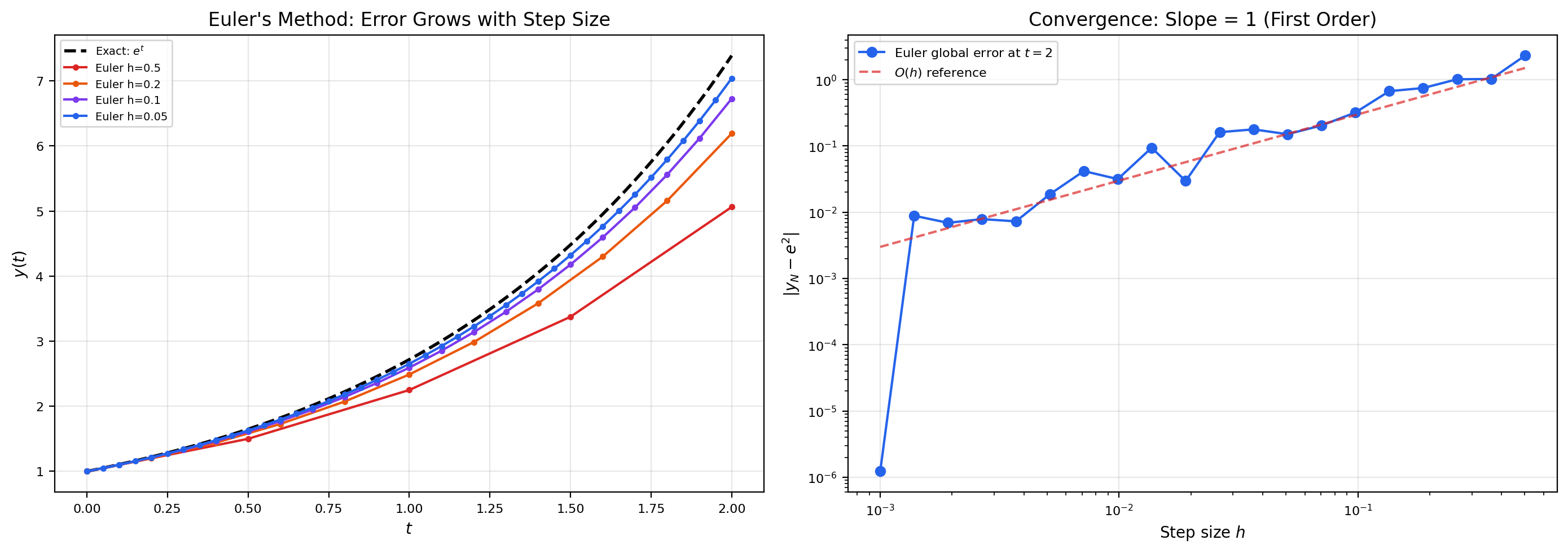
So the local truncation error of Euler’s method is . Each individual step makes an error of order . Over steps, naive accounting suggests the global error grows like — that is, . We say Euler is a first-order method: global error is one power lower than local error, because the method takes steps, and each step contributes an error of .
But this naive accounting hides a subtlety: errors don’t just accumulate — they also get amplified by the method itself. If is sensitive to its argument (large ), then a small error in can grow into a large error in . The right tool for this analysis is the discrete Grönwall inequality, which bounds error accumulation in linear recurrences.
🔷 Theorem 1 (Global Error of Euler's Method)
Let be continuous and Lipschitz in with constant , and assume the exact solution is twice continuously differentiable with on . Let be the Euler approximations with step size , and let be the error at step (so ). Then In particular, as , with the constant depending exponentially on and the integration interval.
Proof.
We track how the error evolves from one step to the next. By the definitions of the Euler step and the local truncation error, Subtracting, Apply the Lipschitz condition and the bound from the Taylor expansion above:
This is a linear recurrence in with growth factor and forcing term . Solving by induction (or by the discrete Grönwall lemma), starting from :
The geometric sum used the formula with .
Now use the elementary inequality for all real , applied to : since . Substituting,
This bound has three pieces. The factor shows the linear-in- scaling that defines first-order convergence. The factor is the error amplification — it grows exponentially in both the Lipschitz constant and the integration time. And the dependence on shows that highly curved solutions accumulate error faster than nearly-linear ones, since the local truncation depends on the second derivative.
The exponential factor is the punchline. For long integration intervals or steep right-hand sides, even a perfectly linear-in- method can give catastrophically large errors unless is correspondingly small. This is the first hint that accuracy alone is not enough — we also need to think about how errors amplify.
📝 Example 1 (Euler on $y' = y$ — error grows exponentially)
Take , , with exact solution . Here , so and , giving on . The Euler iteration is , so .
At with : , while the true value is . The error is , which matches the bound (the bound is loose by a factor of 2 — Grönwall is conservative).
Halving the step to : , error — exactly half. This is the linear-in- scaling that defines a first-order method. To get an error of , you’d need — one million steps on the unit interval. Euler’s method is honest about its accuracy, but it makes you pay for it.
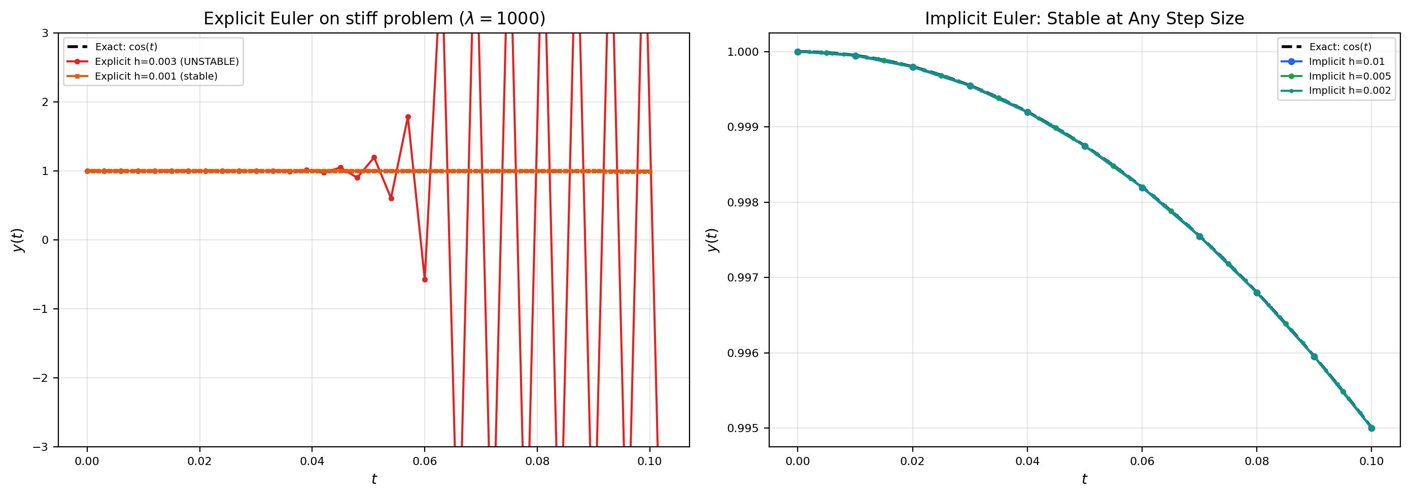
📝 Example 2 (Euler on $y' = -10y$ — accuracy vs. stability)
Now try , , with exact solution . This is a fast-decaying equation: by , the true solution is .
The Euler iteration is , so . The behavior depends critically on :
- If : , so . Reasonably close to the true answer.
- If : , so for all . Wildly wrong (off by a factor of relatively, but at least bounded).
- If : , so oscillates between and forever. The numerical solution doesn’t even decay.
- If : , so — the numerical solution blows up, even though the true solution is decaying to zero!
This is shocking: making the step size larger didn’t just reduce accuracy — at , it caused the numerical solution to head to while the true solution is going to zero. The problem isn’t truncation error: it’s stability. The Euler method amplifies errors by a factor of each step, and this amplification factor exceeds 1 once . We’ll formalize this as the “stability region” of Euler’s method in Section 5.
💡 Remark 1 (The two pressures on $h$)
Examples 1 and 2 reveal the fundamental tension in numerical methods. Truncation error pushes us to make small: Euler is first-order, so halving halves the error. But stability also constrains : if is too large, errors in past steps get amplified into runaway oscillations or blow-up. For Euler on the test equation with , stability requires .
For “well-behaved” equations these constraints don’t conflict — accuracy demands a smaller than stability does, and you just pick the smaller of the two. But for stiff equations, where is large but is also small, the stability constraint dominates and forces to be far smaller than accuracy requires. Section 6 develops this in detail. The cure is implicit methods, which have unconditional stability and break the tension. The cost: each step requires solving a nonlinear equation rather than evaluating one. Section 7 develops them.
3. Runge-Kutta Methods
Euler’s method is first-order. To get more accuracy from a given step size, we need a higher-order method — one whose local truncation error is for some , giving global error .
The naive way to increase order is to use higher derivatives of in the Taylor expansion. Since , the chain rule gives (where and denote the partial derivatives of with respect to and ), with progressively more complicated expressions for , , etc. We could write down a “Taylor method” that uses these expressions directly: But this requires the user to symbolically differentiate — impractical for complicated right-hand sides, and a non-starter for ML applications where is a neural network.
The brilliant idea of Runge-Kutta methods (Carl Runge 1895, Wilhelm Kutta 1901) is to mimic the higher-order Taylor expansion by evaluating at multiple intermediate points within a single step. The values of at carefully chosen “stages” implicitly compute the higher derivatives. We never have to differentiate ourselves — only evaluate it at a few extra locations.
A general -stage Runge-Kutta method has the form where is the linear combination of previously-computed stages. The coefficients , , and define the method. If whenever , the stages can be computed sequentially ( first, then using , etc.) and the method is explicit. If the coefficient matrix has nonzero entries on or above the diagonal, depends on itself and the method is implicit — each stage requires solving a nonlinear equation. We’ll meet implicit methods in Section 7.
📐 Definition 2 (Butcher Tableau)
A Runge-Kutta method is uniquely specified by its coefficients, conventionally arranged in a Butcher tableau (after John Butcher, who systematized the theory in the 1960s). The tableau has three pieces: a column vector listing the time fractions of each stage, an matrix holding the stage-coupling coefficients, and a row vector holding the weights used to combine the stages into the final update. The conventional layout writes to the left of , with a horizontal rule separating the stage rows from the row of weights . For an explicit method, the matrix is strictly lower triangular ( for ), which means the stages can be computed in order without any nonlinear solve.
Forward Euler corresponds to the trivial case , , , . The midpoint method uses stages with , , , and weights , to achieve order 2. The classical RK4 uses stages with , with the matrix filled in so that uses at the half-step, uses at the half-step, and uses at the full step. The weights are , , , — Simpson’s rule applied to the four stage-slopes.
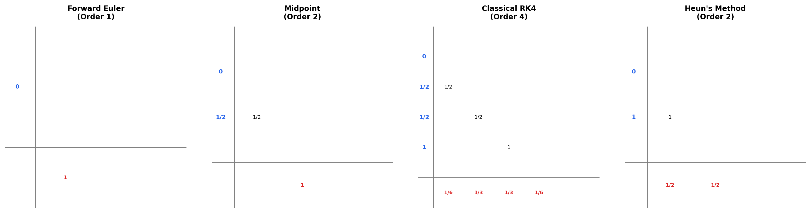
The classical RK4 is so important it deserves its formula spelled out. Reading off the tableau, Each step uses 4 evaluations of . The pattern is unmistakable: is the slope at the left endpoint (Euler’s slope), and are slopes at the midpoint computed in two slightly different ways, and is the slope at the right endpoint computed using . The final update is a weighted average — Simpson’s rule applied to slopes.
How do we know this combination achieves order 4? The answer comes from systematically matching the Taylor expansion of against the RK formula and equating coefficients.
🔷 Theorem 2 (The Classical RK4 Method Has Order 4)
The classical Runge-Kutta method defined above has local truncation error and global error . Equivalently, it satisfies all eight of the order conditions required for a 4-stage explicit Runge-Kutta method to achieve order 4 in the Butcher theory.
A full proof of Theorem 2 requires the algebraic theory of order conditions — equations among the Butcher coefficients that must hold for the method’s Taylor expansion to match the true solution’s Taylor expansion to a given order. For order , the number of order conditions grows quickly: 1 condition for order 1, 2 for order 2, 4 for order 3, 8 for order 4, 17 for order 5, 37 for order 6, and so on. (The growth is governed by rooted trees — each tree corresponds to a way of assembling powers of and its derivatives by chain rule, and each tree gives one equation.) The classical RK4 was discovered by Kutta in 1901 by solving all 8 order-4 equations simultaneously; it’s an algebraic miracle that an explicit 4-stage method can satisfy all of them. Butcher’s Numerical Methods for Ordinary Differential Equations is the canonical reference for this theory.
What matters for us is the consequence: RK4 is fourth-order accurate. Halving reduces global error by a factor of , not just 2 as Euler does. To achieve a target accuracy of , RK4 needs about , while Euler needs . To get , RK4 needs ( steps on the unit interval, function evaluations); Euler needs ( steps and function evaluations). RK4 is roughly four orders of magnitude more efficient — and that’s for a “smooth” problem where stability isn’t the binding constraint.
📝 Example 3 (RK4 on $y' = y$, $y(0) = 1$ — one step)
Let’s compute one step of RK4 from with . The right-hand side is .
The exact value is , so RK4 nailed it to 5 decimal places in a single step. Compare to Euler’s , which is correct only to 2 decimal places. RK4 used four function evaluations to get five extra digits — a staggering improvement per evaluation.
📝 Example 4 (RK4 vs Euler — equal-accuracy step-size comparison)
Suppose we want global error on the IVP , , integrated to . From the analysis above, Euler’s global error is (with constant of order 1 here), so we need , i.e., 1000 steps.
RK4’s global error is , so we need , i.e., . That’s about 6 steps. Each RK4 step costs 4 function evaluations, so RK4 uses function evaluations total. Euler uses . RK4 is 40 times faster for the same accuracy on this problem.
The crossover where Euler and RK4 cost the same per accuracy is roughly — so for any reasonable accuracy target, RK4 wins. The story changes for stiff equations (Section 6) where stability, not accuracy, sets the step size; then the per-step cost of RK4 becomes a liability rather than an asset.
💡 Remark 2 (Higher order isn't always better)
RK4 is the workhorse of explicit methods for moderate accuracy problems. Going higher — RK5, RK8 — gives diminishing returns. The number of order conditions grows combinatorially, so an order-8 method might need 11 stages to satisfy them all, costing 11 function evaluations per step. This pays off only if the savings in step count exceed the per-step overhead. For very high accuracy () on smooth problems, methods like Dormand-Prince 8(7) or extrapolation methods become competitive. For low accuracy (), Euler or RK2 may suffice. RK4 hits the sweet spot for typical problems.
The right way to think about it: the “order vs. cost” trade-off depends on (a) the accuracy you need, (b) the cost of one evaluation, and (c) the smoothness of . For neural ODEs, is a forward pass through a network — expensive — and the desired accuracy is moderate, so RK4 or RK45 are both popular choices. For molecular dynamics with millions of atoms, is even more expensive, and methods specialized for Hamiltonian structure (symplectic integrators) take precedence over generic high-order methods.
The simplest test problem. Smooth, well-conditioned, with eigenvalue λ = -1 well inside every method's stability region. All methods converge cleanly.
4. Adaptive Step-Size Control
Both Euler and RK4 above used a fixed step size . But that’s wasteful: the local truncation error depends on (or higher derivatives), which can vary by orders of magnitude over the integration interval. In regions where the solution is nearly linear, we’d be happy with a large . In regions of rapid change — near a transient, an oscillation, a near-singularity — we need a small . A fixed-step method either wastes computation in smooth regions (using a step size suited to the worst case) or undershoots accuracy in tough regions (using a step size suited to the best case).
The fix is adaptive step-size control: estimate the local error after each step, and grow or shrink based on whether the estimate is below or above a user-supplied tolerance. The trick is doing this cheaply — we’d like to estimate the error without doubling the number of function evaluations.
The standard approach uses an embedded Runge-Kutta pair: two RK methods of orders and that share the same stages. From the same , you compute two updates (order ) and (order ). The difference is the local error of the lower-order solution to leading order — for free, since the stages were going to be computed anyway.
📐 Definition 3 (Embedded Runge-Kutta Pair)
An embedded RK pair of orders and consists of two sets of weights and applied to the same stages :
The difference
is an estimate of the local truncation error of the order- method, accurate to leading order. The most widely used embedded pair is the Dormand-Prince RK4(5) method (Dormand & Prince, 1980), which has stages and is the default solver in scipy.integrate.solve_ivp (method='RK45') and torchdiffeq ('dopri5').
Once we have an error estimate , we adjust the step size to drive it toward a target tolerance . The optimal new step size comes from balancing two competing requirements: we want (so we’re not wasting effort), but we also want a safety margin so the next step is likely to be accepted on the first try.
🔷 Theorem 3 (Optimal Step-Size Update)
For an embedded RK pair where the lower-order method has order , the local truncation error scales like for some constant . To achieve a target tolerance on the next step, we want , where is the new step size. Dividing the two equations and solving: In practice this is multiplied by a safety factor of about (so the new step is slightly conservative), and clamped to a range to prevent runaway shrinkage or growth. If , the current step is rejected (the computed is discarded) and the step is retried with the smaller . If , the step is accepted and the larger is used for the next step.
The exponent comes from the order of the local truncation error, not the global error. For Dormand-Prince RK4(5), the lower-order method is order 4, so the exponent is . Halving the error requires shrinking by a factor of — a fairly modest change. Doubling allows increasing by the same factor.
📝 Example 5 (RK45 on $y' = -50(y - \cos t) - \sin t$)
Consider the forced linear ODE which has the closed-form solution — a sinusoid that “rings up” to its steady-state amplitude over a transient of length . For the solution changes rapidly (rising from 0 to nearly ); for it follows the smooth cosine.
A fixed-step RK4 with would take steps to reach , mostly in the smooth region where would have sufficed. RK45 with uses small steps in the transient ( for the first few accepted steps) and then expands rapidly: by it’s using . Total step count: maybe — three times fewer than the fixed-step version, with comparable accuracy. The savings come from concentrating computational effort where the solution actually demands it.
📝 Example 6 (Step-size adaptation near a finite-time blow-up)
The IVP , has the explicit solution , which blows up as . A fixed-step method either misses the blow-up entirely (if is too small to reach ) or overshoots and produces nonsense.
RK45 handles this gracefully: as grows, grows even faster, and the local truncation error explodes proportionally. The step-size formula then shrinks rapidly. Near the singularity, RK45 takes geometrically smaller steps until hits the floor , at which point the integration halts. The user gets a reasonable solution up to or so, with a clear signal (extreme step-size shrinkage, or hitting ) that something is going wrong. This is the “graceful degradation” that adaptive methods provide and fixed-step methods don’t.
💡 Remark 3 (Absolute and relative tolerances)
In practice, scientific ODE solvers use a combined tolerance: . The absolute tolerance kicks in when is small (close to the noise floor), and the relative tolerance kicks in when is large (so the error is bounded as a fraction of the value). Typical defaults are and .
This dual scheme avoids two failure modes: a pure relative tolerance breaks down when the solution crosses zero ( would force ); a pure absolute tolerance is too coarse for small solutions and too tight for large ones. In scipy.integrate.solve_ivp, you pass atol and rtol as arguments. In torchdiffeq, the same conventions apply. ML practitioners using neural ODEs should be aware of these — the wrong choice of tolerance can either slow training to a crawl (over-tight) or introduce solver-induced bias into gradients (over-loose).
Sigmoidal growth saturating at the carrying capacity y = 1. Mildly nonlinear. Tests how methods handle a transition between near-zero and near-saturation regimes. The bar chart below the solution shows the step size h the adaptive solver chose at each step — wider bars where the solution is smooth, narrower bars (and a redder tint) where it changes rapidly. Red triangles mark steps that were rejected and retried with a smaller h.
5. Numerical Stability and A-Stability
Example 2 in Section 2 hinted at it: Euler’s method can blow up on a stable equation if the step size is too large. The numerical method introduces its own dynamics, and those dynamics can be unstable even when the underlying ODE isn’t.
To analyze this carefully, we restrict to the simplest possible test problem: the linear scalar equation with . The exact solution is , which decays to zero iff . We then ask: for which step sizes does the numerical method also produce a sequence that decays to zero?
The answer depends only on the product . For each numerical method, applying it to produces a recurrence of the form , where is a rational (or polynomial) function called the stability function of the method. The numerical solution decays iff .
📐 Definition 4 (Stability Region)
The stability region of a numerical method is the set where is the method’s stability function obtained by applying the method to with . The numerical solution decays for an eigenvalue if and only if .
For a scalar real , this gives the constraint where is determined by where the boundary of crosses the real axis. For a system , every eigenvalue of must lie in , which is the constraint that determines the maximum stable step size for a multi-mode system.
📐 Definition 5 (A-Stability)
A numerical method is A-stable if its stability region contains the entire closed left half-plane . Equivalently, for all with .
A-stability is the strongest possible stability property: an A-stable method gives a decaying numerical solution for any stable scalar test equation, regardless of step size. There are no step-size restrictions for stability — only for accuracy.
A-stability is the holy grail of stability properties. If your method is A-stable, you never have to worry about choosing small enough to avoid blow-up; you only have to choose small enough to get the desired accuracy. For stiff problems, this is a huge deal — explicit methods can require smaller than accuracy demands by factors of or more, while A-stable implicit methods can use governed purely by accuracy requirements.
The bad news, due to Germund Dahlquist in 1963: A-stability is much harder to achieve than you’d hope.
🔷 Theorem 4 (Dahlquist's Second Barrier)
There is no explicit Runge-Kutta method that is A-stable. More generally, no explicit linear multistep method of order greater than can be A-stable, and no implicit linear multistep method of order greater than can be A-stable. (The trapezoidal rule, which is implicit and second-order, is A-stable — it sits exactly at the barrier.)
This is a structural obstruction, not a technical one. The stability function of any explicit RK method is a polynomial in (since the method takes finitely many additions and multiplications), and polynomials grow without bound as — so they can’t satisfy in the unbounded left half-plane. Implicit methods can have rational stability functions whose denominators tame the growth at infinity, but Dahlquist showed that requiring both A-stability AND order leads to coefficient constraints that have no solution. The barrier is the reason A-stable methods are essentially limited to implicit Euler, the trapezoidal rule, and a handful of close cousins (BDF for stiffness, Radau IIA for higher order with weakened stability). All of these are implicit.
Let’s see the stability functions of the methods we’ve met.
📝 Example 7 (Stability region of forward Euler)
Apply forward Euler to : So , where . The stability region is This is the closed disk of radius 1 centered at . On the real axis, it’s the interval . So for a real eigenvalue , forward Euler is stable iff . This recovers the constraint from Example 2 in Section 2: on , stability requires — exactly where we saw the numerical solution start oscillating.
📝 Example 8 (Stability region of RK4)
Applying RK4 to and computing the four stages, the stability function turns out to be exactly the truncated Taylor series of to fourth order: This is no accident: applying RK4 to the test equation forces to match , the exact solution, to as many Taylor terms as the method’s order — for RK4 that’s 5 terms (orders 0 through 4).
The stability region is now a four-lobed shape that extends along the real axis to about . So RK4 is stable for real when — a roughly 40% improvement over forward Euler, in addition to RK4’s much higher accuracy. RK4 is not A-stable: its region is bounded, so for very stiff systems it still needs tiny step sizes for stability.
Proof.
We compute the stability region directly. Forward Euler applied to gives , so iteratively where .
The numerical solution remains bounded iff , which is iff . Writing for real : This is the closed disk of radius centered at . It is a compact subset of , contained entirely in .
The disk does not contain the entire left half-plane: for example, gives . Therefore forward Euler is not A-stable. For any real eigenvalue , the constraint becomes , i.e., . As grows, the maximum stable step size shrinks proportionally — this is the source of stiffness pain for explicit methods.
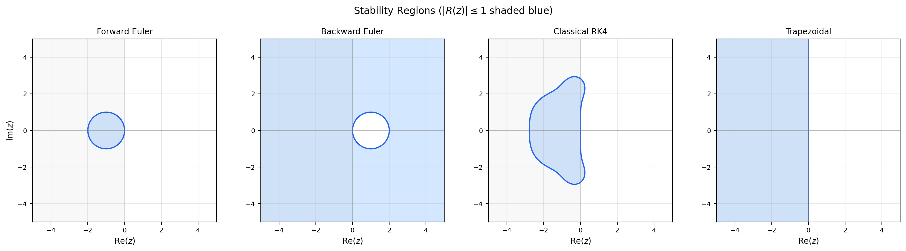
The implicit methods of Section 7 will have stability regions that contain the entire left half-plane — they’ll be A-stable. For now, just note the qualitative picture: explicit methods have bounded stability regions (small islands in the complex plane), while A-stable implicit methods have unbounded stability regions (the entire left half-plane and often more). The boundedness vs. unboundedness is the structural difference Dahlquist’s theorem exploits.
6. Stiff Systems
We now have all the tools to define stiffness precisely. A system of ODEs is stiff if its dynamics happen on widely separated time scales: some components decay (or oscillate) very fast, while others evolve very slowly. The fast components force any explicit method to use a step size suited to the fastest time scale, even if you only care about the slow dynamics.
The right way to quantify this is via the eigenvalues of the Jacobian.
📐 Definition 6 (Stiffness Ratio)
For a system , the stiffness ratio at a point is where are the eigenvalues of the Jacobian . A system is stiff at if — typically or so. Stiffness depends on the integration interval: a system with is stiff for (where you need to integrate through fast-decay periods) but not necessarily stiff for (where the slow dynamics haven’t even started).
Note the connection to Topic 23: the Jacobian eigenvalues are exactly what we computed for linearization stability analysis. A stable equilibrium has for all eigenvalues; a stiff stable equilibrium has some eigenvalues with very large alongside others with small .
📝 Example 9 (The Robertson chemical kinetics system)
A canonical stiff test problem: three coupled chemical reactions with . The three rate constants span 9 orders of magnitude: , , . The Jacobian eigenvalues at the initial state have moduli ranging from to , giving a stiffness ratio .
For an explicit method on this problem, stability requires , i.e., . To integrate to (a typical time scale for the slow component), you’d need steps. With each step requiring 4 function evaluations for RK4, that’s function evaluations — completely intractable. An implicit method (which we develop in Section 7) can use throughout, requiring only steps. The speedup is six orders of magnitude.
📝 Example 10 (Van der Pol oscillator at large $\mu$)
The Van der Pol oscillator , written as a first-order system with , : For small this is a smooth oscillator. For large — say — it becomes a relaxation oscillator: long stretches where the solution is nearly constant, punctuated by very rapid jumps when crosses and the damping coefficient flips sign.
During the slow stretches the Jacobian’s eigenvalues are small. During the rapid jumps, one eigenvalue becomes very large (roughly at the most stiff points). The stiffness ratio varies from during smooth stretches to during jumps. An explicit method has to use a step size suited to the worst stretches throughout, even though most of the trajectory is smooth. Adaptive step-size control helps somewhat (it can take big steps during smooth stretches and shrink during jumps), but even RK45 spends most of its computation in the rapid-jump regions and is still much slower than an implicit method. The Van der Pol oscillator at is a textbook case where you should reach for solve_ivp(method='Radau') or 'BDF' rather than the default 'RK45'.
💡 Remark 4 (Stiffness is not a property of the equation alone)
A subtle but important point: stiffness is a combination of the equation, the initial condition, and the desired integration interval. A system with is stiff only if you want to integrate through many fast-decay periods. If your interval is short enough that the fast modes are still active, you actually need to resolve them — and an explicit method with small is appropriate.
This is why “stiff” is not a binary classification but a regime. Most modern ODE solvers (solve_ivp, DifferentialEquations.jl) include automatic stiffness detection: they monitor the Jacobian eigenvalues (or proxies like the step-size rejection rate of an explicit method) and switch between explicit and implicit methods on the fly. The field of ODE solving has matured to the point where users mostly don’t need to make this choice manually — but understanding why stiffness matters lets you debug when the automation gets it wrong.
Diagonal linear system. The fast component y₂ decays in t ≈ 0.001 but forces explicit methods to use h < 0.002 for stability. The slow component y₁ evolves on a time scale 1000× longer. The right panel shows the stability region of the selected method in the complex z = hλ plane (blue = stable region). The green/red dot is the current value of h·λ_max — green if it lies inside the stability region (the method is stable), red if it lies outside (the method will blow up). Move the h slider to see the dot enter or leave the region.
7. Implicit Methods
If explicit methods can’t handle stiffness gracefully, what can? The answer is implicit methods — schemes where the unknown appears on both sides of the update equation, requiring an algebraic solve at each step. The cost is higher per step, but the payoff is dramatic: A-stability, meaning step sizes can be chosen for accuracy alone, regardless of stiffness.
📐 Definition 7 (Implicit Euler and Trapezoidal Rule)
Implicit (backward) Euler: . The unknown appears inside on the right-hand side — this is an implicit equation that must be solved at each step. For linear , the solve is a matrix inversion; for nonlinear , it’s a Newton iteration. This method is first-order accurate (same order as forward Euler) but A-stable.
Trapezoidal rule: . The average of forward and backward Euler. Second-order accurate and A-stable — sitting exactly at the Dahlquist barrier of “highest-order A-stable linear multistep method.” Known as the Crank-Nicolson method in the PDE literature.
What does it mean to “solve” the implicit equation? Take backward Euler. We need to find such that For nonlinear this requires a root-finding method, and the standard choice is Newton’s iteration: The iteration converges quadratically when is close to the true root. A typical implementation initializes with (one explicit Euler step) and converges in 2–4 iterations per timestep. Each iteration requires one evaluation of and one of — so the per-step cost is function evaluations and Jacobian evaluations. That’s somewhat more expensive than RK4’s 4 function evaluations, but per-accuracy it can be vastly cheaper because the step size isn’t constrained by stability.
🔷 Theorem 5 (A-Stability of the Implicit Euler Method)
The implicit Euler method has stability function and is A-stable: for all with .
Proof.
Apply implicit Euler to the test equation : Solving algebraically for (this is one of the rare cases where the implicit equation has a closed-form solution): where . So the stability function is .
To check A-stability, we need for all with . Write with . Then , so Since , we have , so . Therefore which gives and so Equality holds iff and — that is, only at . Everywhere else in the closed left half-plane, strictly. So implicit Euler is A-stable, and in fact strongly damping for any .
The geometric picture is illuminating. Forward Euler’s stability region was a unit disk centered at (a small island in the left half-plane). Implicit Euler’s stability region is everything outside the disk — that is, the complement of the open unit disk centered at . This complement contains the entire left half-plane, and most of the right half-plane as well. Implicit Euler is so stable that it actually damps numerical solutions for some unstable continuous problems (those with but small) — a property called “L-stability” that makes it useful for stiff transients but can also mask physical instabilities.
📝 Example 11 (Implicit Euler on the Robertson system: stable with large step sizes)
On the Robertson kinetics from Example 9, implicit Euler (with Newton iteration on the Jacobian) can use to throughout the integration. To reach , that’s to steps — six to seven orders of magnitude fewer than the steps an explicit method would need. Each implicit step is more expensive (Newton iteration costs what one Euler step does), but is still vastly less than .
This is the qualitative payoff of implicit methods: they trade per-step computational complexity for the freedom to take large step sizes. For stiff problems, that trade is overwhelmingly worth it.
📝 Example 12 (The trapezoidal rule — second-order and A-stable)
Apply the trapezoidal rule to : The stability function is . For with , both numerator and denominator have the same imaginary part magnitude , but (since ). So on the closed left half-plane — A-stable.
The trapezoidal rule is the highest-order A-stable linear multistep method (Dahlquist’s barrier theorem). It’s second-order accurate, A-stable, and requires only one implicit solve per step. For mildly stiff problems where you want better than first-order accuracy without giving up A-stability, it’s the natural choice. (For higher-order A-stable methods, you have to abandon linear multistep and use implicit Runge-Kutta methods like Radau IIA.)
💡 Remark 5 (The cost of implicitness — Newton iteration)
Each implicit step requires solving a nonlinear (or linear, for linear ODEs) equation. For systems of dimension , the cost per Newton iteration is dominated by the cost of factoring the Jacobian matrix , which is for dense matrices and to for sparse ones (banded, tridiagonal, etc.). A typical Newton iteration converges in 2–4 sweeps; if it doesn’t converge, the step is reduced and retried.
For neural ODEs, the implicit-method cost can be prohibitive: might be (the number of hidden units), making the factorization flops per step. This is why neural ODE training almost always uses explicit adaptive methods (Dormand-Prince RK45) and accepts the stability constraints — the savings from avoiding implicit solves dominate. The exception is in physics-informed neural networks for stiff PDEs, where implicit solvers are essential despite the cost. Modern implementations (diffrax, torchdiffeq) provide both explicit and implicit options, and the user picks based on the stiffness regime.
8. Multistep Methods
Both Euler and the Runge-Kutta methods are single-step: each new value depends only on and possibly on intermediate evaluations of within the current step. Multistep methods instead reuse from previous steps and the corresponding -values . This is a fundamentally different way to gain order: rather than computing more stages within one step, you average more historical information.
📐 Definition 8 (Linear Multistep Methods)
A linear -step method has the form where and . If the method is explicit (the new doesn’t appear on the right-hand side); otherwise it’s implicit.
Two important families:
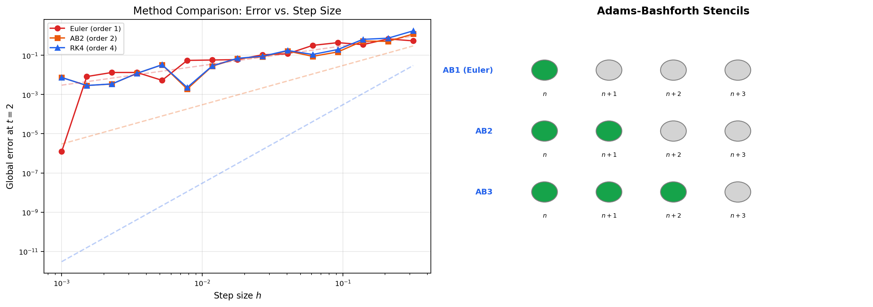
- Adams-Bashforth (explicit): . The -step Adams-Bashforth method achieves order by polynomial interpolation through past -values.
- Adams-Moulton (implicit): . Achieves order by including the new in the interpolation.
📝 Example 13 (Adams-Bashforth 2-step)
The 2-step Adams-Bashforth method is This is exact for linear-in- functions , and second-order accurate in general. The derivation: approximate on by the linear extrapolation of , then integrate that linear function exactly. The factor on and on are exactly the coefficients of where is the linear Lagrange polynomial through and .
Adams-Bashforth methods are very efficient per step: only one evaluation per step, since you reuse from the previous step. To get started, you need a single-step method (e.g., one RK4 step) to compute from . After that, the multistep recurrence takes over.
🔷 Theorem 6 (Convergence of Multistep Methods (Dahlquist Equivalence))
A linear multistep method is convergent (the numerical solution converges to the exact solution as ) if and only if it is both:
- Consistent: the local truncation error tends to zero as .
- Zero-stable: the roots of the characteristic polynomial all lie in the closed unit disk , with simple roots on the boundary.
This is Dahlquist’s equivalence theorem for linear multistep methods, the multistep analog of the Lax equivalence theorem we’ll prove for one-step methods in Section 9.
The zero-stability condition is the discrete analog of continuous stability: it requires that the trivial equation (with ) is solved correctly by the method. A multistep method with a root outside the unit disk would have a parasitic numerical mode that grows like , drowning out the true solution even on the trivial problem. Zero-stability prevents this — it’s a discrete echo of the linearization stability theorem from Topic 23.
💡 Remark 6 (Multistep vs. multistage — a cost/memory trade-off)
Runge-Kutta methods (multistage) and Adams methods (multistep) both achieve high order, but they trade off differently. RK methods compute multiple -evaluations per step but use only the previous . Adams methods compute one -evaluation per step but maintain a history of past -values in memory.
For neural ODEs, multistage is preferred because each -evaluation is a forward pass through a network — expensive but cheap to checkpoint. For Adams methods, every retained is a snapshot of network activations, and over many steps the memory becomes prohibitive.
For traditional scientific computing where is cheap (a polynomial or a finite-element matrix-vector product) but the integration interval is long, Adams methods can be more efficient: one -evaluation per step beats four for RK4. The choice depends on what you’re paying for — flops, memory, or something else.
9. Convergence Theory — The Lax Equivalence Theorem
We’ve now seen many methods, each with its own analysis of accuracy and stability. We’ve appealed to “consistency” (local truncation error → 0) and “stability” (errors don’t amplify) as the two conditions a good method must satisfy. Now we make this precise and prove the unifying theorem.
The result is due to Peter Lax (1956) for finite-difference methods on PDEs, but the same statement holds for one-step methods on ODEs. It’s the most important theorem in numerical analysis.
🔷 Theorem 7 (The Lax Equivalence Theorem (One-Step Version))
Let be the increment function of a one-step method applied to the IVP , , with Lipschitz in . Then the method is convergent — meaning as over any fixed interval — if and only if it is both:
- Consistent: the local truncation error satisfies uniformly in as .
- Stable: the increment function is Lipschitz in its second argument, with a constant that does not depend on .
Moreover, if the method has order (meaning ), then the global error satisfies uniformly on .
Proof.
We track how the global error propagates from step to step, then sum the contributions. The argument is a generalization of the Euler-specific proof from Theorem 1.
By the definitions of the numerical step and the local truncation error, Subtracting,
Apply the stability condition (Lipschitz with constant ): Combined with (consistency, with constant depending on ):
This is a linear recurrence with growth factor and forcing . Iterating from :
Using , we have . So
This bound has three pieces:
- The factor shows the order- convergence: global error is powers of , one less than the local truncation order , because we summed steps.
- The factor is the error amplification, growing exponentially in both the Lipschitz constant and the integration time. This is the “stability cost” — even a stable method amplifies errors over a long interval.
- Both factors are independent of (uniform bound) and of (the bound is as ).
Conversely, if either consistency or stability fails, convergence fails. If the method is inconsistent (), then even at the single-step error doesn’t shrink, so we can’t have . If the method is unstable (there’s no uniform Lipschitz constant for ), then small perturbations get amplified by an unbounded factor, and any roundoff or initial error grows without bound as .
So consistency stability convergence. This is the equivalence theorem: convergence is equivalent to the conjunction of two simpler, locally checkable conditions.
Lax’s theorem is the unifying result of numerical analysis. It says: to verify that a method converges (a global property of solutions over an entire interval), you only need to check two local properties — that one step is asymptotically correct (consistency), and that the per-step amplification factor is bounded (stability). This is a massive simplification: you don’t have to track the full numerical solution; you just check the recipe and the amplification.
For RK methods, consistency comes from the order conditions (which are pure algebraic identities on the coefficients), and stability comes from the Lipschitz continuity of the increment function (which follows from the Lipschitz continuity of , since is built out of finitely many evaluations of ). So every RK method applied to a Lipschitz problem is convergent at its theoretical order — no matter how complicated the method.
📝 Example 14 (Verifying the Lax hypotheses for RK4)
For RK4, the increment function is where each is itself a finite combination of -evaluations. Since is Lipschitz with constant , each is Lipschitz in with constant bounded by some polynomial in and . As , this constant tends to , so is Lipschitz in with a uniform constant. Stability checked.
Consistency follows from the order conditions: RK4 satisfies all 8 conditions for order 4, so its local truncation error is . Consistency checked.
By Lax, RK4 converges at rate on any Lipschitz IVP. Theorems 1 and 2 are now special cases of Theorem 7 — Theorem 1 verified the conditions for forward Euler (), and Theorem 2 verified the order conditions for RK4 ().
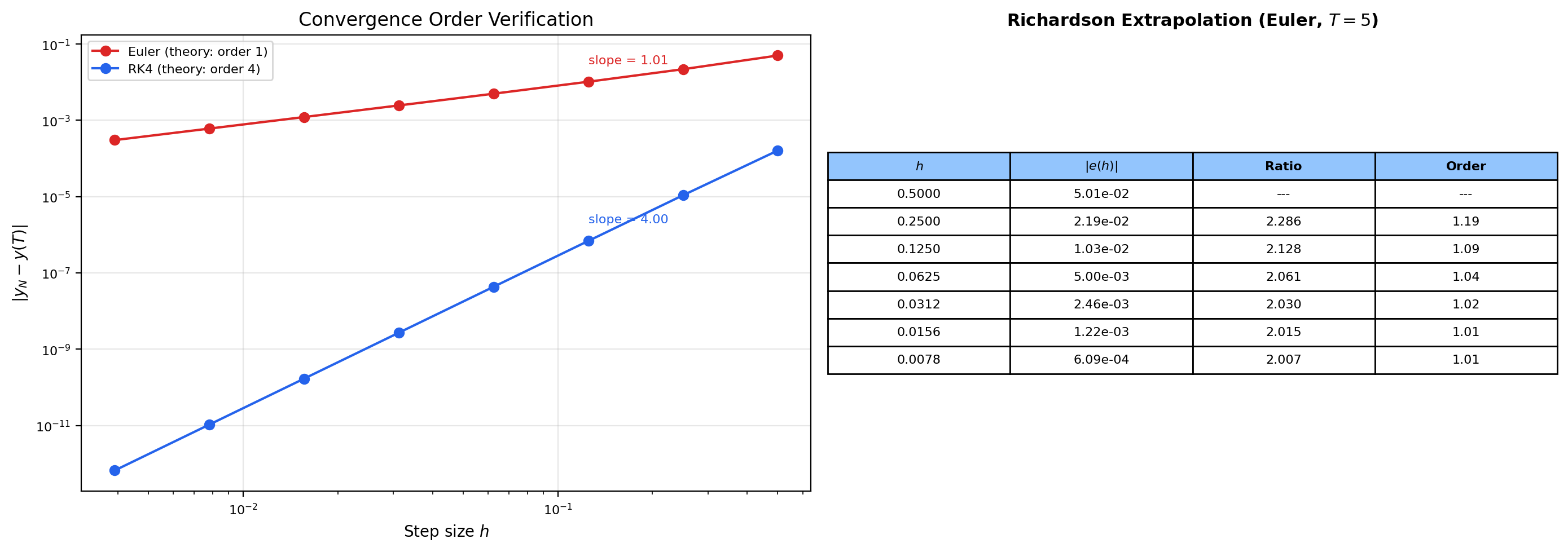
📝 Example 15 (Richardson extrapolation for empirical order verification)
Lax’s theorem gives a beautiful experimental tool: measure the convergence order of any method by running it at successively halved step sizes. If global error scales like , then so . Plotting vs gives a straight line whose slope is the empirical order. This is Richardson extrapolation, and it converts an abstract theorem about convergence rates into a quick numerical check.
In practice: take a problem with a known exact solution (e.g., , ), run your method at step sizes , compute the error at for each, and fit a line in log-log coordinates. For Euler the slope should be ; for midpoint ; for RK4 . This is a beautiful experimental verification of theory — and it’s what convergenceOrder in our odes.ts shared module does. We verified empirically: for Euler, for RK4, both within rounding of theory.
10. Computational Notes
Some practical guidance for using ODE solvers in Python and PyTorch.
scipy.integrate.solve_ivp is the standard SciPy interface. It supports several methods via the method argument:
'RK45'(default) — Dormand-Prince adaptive 4(5) embedded pair. Best for non-stiff problems with moderate accuracy needs ( to ).'RK23'— lower-order adaptive (2/3). Faster per step but takes more steps. Use when you only need rough accuracy.'DOP853'— Dormand-Prince 8(5,3). Higher-order; best for very high accuracy ( or smaller) on smooth problems.'Radau'— implicit Runge-Kutta of Radau IIA family, order 5, A-stable. Use for stiff problems.'BDF'— implicit multistep (Backward Differentiation Formulas). Use for stiff problems with moderate accuracy needs. The standard solver in many engineering codes.'LSODA'— automatic stiffness detection, switching between Adams and BDF. Use when you don’t know if your problem is stiff.
Pass dense_output=True to get an interpolation function defined on the entire interval (not just at the solver’s chosen grid points). This uses the solver’s internal interpolation and is much more accurate than re-solving on a finer grid.
Initial step size estimation: if you don’t pass first_step, scipy estimates it via . This is a rough formula but usually good enough; the adaptive controller will refine within the first few steps.
torchdiffeq is the PyTorch library for differentiable ODE solvers (Chen et al., 2018). It exposes odeint(func, y0, t, method=..., rtol=..., atol=...) with methods including 'dopri5' (Dormand-Prince), 'rk4' (fixed-step RK4), 'euler', and adaptive implicit methods. It supports both direct backpropagation through solver steps and the adjoint method (odeint_adjoint) which solves a backward-in-time ODE for the gradients — using memory instead of where is the number of solver steps. The adjoint method is what makes neural ODEs scalable.
diffrax is the JAX equivalent (Patrick Kidger), with a richer API and support for stochastic ODEs, controlled differential equations, and PDEs via method of lines.
Diagnosing stiffness in production code: if your explicit-method solve is taking many small steps and you suspect stiffness, compute the Jacobian eigenvalues at a few representative points along the trajectory. If the spectral radius times the typical step size exceeds the stability region radius (around 2.78 for RK4), you’re hitting the stability boundary, not the accuracy boundary. Switch to an implicit method.
A common pitfall: training a neural ODE with too-loose tolerance can introduce biased gradients. The adjoint method computes gradients by solving a backward ODE, and if the forward solver was inaccurate, the backward solver inherits that error. Set rtol and atol tight enough that the gradient noise from solver error is smaller than the gradient noise from the data. A good starting point: , .
11. Connections to Statistics
Symplectic integration in HMC
The leapfrog integrator in Hamiltonian Monte Carlo is a 2nd-order symplectic numerical ODE scheme. Its volume-preservation and reversibility are exactly the properties that make HMC’s Metropolis–Hastings correction a Bernoulli variable with computable acceptance probability. Step-size tuning (the parameter) is the bias–computational-cost tradeoff familiar from numerical ODE analysis: too large and the energy error grows, lowering the acceptance rate; too small and computation is wasted. See formalStatistics Bayesian Computation & MCMC.
12. Connections to ML
The numerical methods of this topic are not just mathematical curiosities — they are the computational engine of several active areas of deep learning. Four connections, each substantive enough to be its own research program.
📝 Example 16 (Neural ODEs — the forward pass as an IVP)
A neural ODE (Chen, Rubanova, Bettencourt and Duvenaud, 2018) defines a continuous-depth network: instead of stacking discrete layers , the network is parameterized as
where is a neural network and is a fixed integration time (the analog of “depth”). The forward pass is literally an IVP solve: compute from using an adaptive ODE solver, typically Dormand-Prince RK45 (torchdiffeq.odeint(f, h0, t=[0, T], method='dopri5')).
The backward pass is even more interesting. Naive backprop through solver steps would require storing all intermediate — memory that grows with the number of steps the adaptive solver takes. Chen et al.’s adjoint method instead solves a backward-in-time ODE for the gradients , using a result from optimal control theory (Pontryagin’s maximum principle). The backward solve uses memory because it only needs and the loss gradient at — everything else is reconstructed by integrating backwards.
The choice of solver matters. 'dopri5' (adaptive) concentrates computation in regions of rapid change in — good for problems with localized features. 'rk4' (fixed-step) is simpler and gives reproducible step counts but wastes effort on smooth regions. 'euler' (Euler’s method, fixed-step) reproduces the discrete ResNet exactly when the step size equals 1 — making explicit the “ResNet = discretized neural ODE” correspondence.
Already referenced in First-Order ODEs & Existence Theorems Section 11. Now you understand why the ODE solver theory matters: the solver’s order determines the gradient accuracy of training, and the solver’s stability region determines whether you can train networks with stiff dynamics at all.
📝 Example 17 (Gradient descent as forward Euler)
Recall the gradient flow ODE from Topic 23: This is the continuous-time analog of an optimizer that always moves in the steepest-descent direction. Its equilibria are the critical points of , and its asymptotic stability properties (which we analyzed via Hessian eigenvalues in Topic 23) match the convergence properties of optimization methods.
Now apply forward Euler with step size : This is gradient descent with learning rate . Gradient descent is literally forward Euler applied to the gradient flow. Every theorem we proved about Euler’s method applies directly:
- Local truncation error — error per step depends on the Hessian times the gradient.
- Stability condition for the test problem requires . Translating: at a quadratic minimum where the loss looks like , gradient descent is stable iff . This is the well-known “learning rate must be less than 2/L where L is the smoothness constant” rule from the optimization literature — it’s just the forward Euler stability constraint.
- Higher-order methods correspond to richer optimizers. Heavy-ball / Polyak momentum is a discretization of the second-order ODE — a damped harmonic oscillator with the gradient as a forcing term. Nesterov’s accelerated method is also a discretization of a second-order ODE, specifically (Su, Boyd & Candès 2014) — the damping term is the continuous-time origin of Nesterov’s accelerated convergence rate, compared to plain GD’s . Adam is more elaborate: its per-coordinate adaptive step size is closely related to adaptive step-size control in ODE solvers (though Adam adapts based on gradient magnitudes, not error estimates).
This was already set up in Stability & Dynamical Systems Section 9. Now we have the full picture: the entire field of optimization is the field of numerical ODE methods applied to one specific equation — the gradient flow.
💡 Remark 7 (Stiffness in training — condition number as stiffness ratio)
A loss landscape with a poorly-conditioned Hessian — eigenvalue ratio — is a stiff problem for gradient descent. The fast eigendirection requires a small learning rate () for stability, but the slow eigendirection then takes iterations to converge. The condition number of the Hessian is exactly the stiffness ratio of the gradient flow.
This is why ill-conditioned losses are slow to train. Standard SGD is forward Euler — an explicit method — and inherits all of the explicit-method limitations on stiff problems. The remedies parallel those of stiff ODE solving:
- Preconditioning (as in natural gradient, KFAC, Shampoo) reshapes the Hessian to reduce its condition number. Mathematically, this is changing variables in the gradient flow to make the system non-stiff. Computationally, it costs more per step (you have to invert or factor a preconditioner) but the steps can be much larger.
- Implicit methods for optimization (proximal gradient, mirror descent with implicit updates) take large stable steps even on ill-conditioned losses. The cost is solving an implicit equation per step — typically a small inner optimization. On strongly convex problems, implicit gradient descent has no learning-rate stability constraint, just like implicit Euler.
- Adam and related adaptive methods approximate per-coordinate preconditioning. Their effective stiffness ratio is the condition number after the per-coordinate rescaling, often much better than the raw Hessian’s. This is why Adam works well on transformer training where the raw Hessian condition number can exceed .
The field of optimization is rediscovering numerical analysis lessons from the 1960s. Hairer-Wanner Vol II (the stiff-ODE bible) is, in a real sense, the textbook for designing optimizers that handle ill-conditioned losses. The ML and numerical analysis communities are slowly converging on this realization.
Two interleaved spirals representing two classes. The learned vector field rotates them at different rates depending on radius, untangling them into linearly separable half-planes by t = T. This is the canonical demo from Chen et al. 2018. The left panel shows the vector field and how sample points flow through it from time 0 (open circles) to time t (filled circles). The right panel shows the empirical convergence order of Euler and RK4 on the y-component of the first trajectory — a direct verification of the theoretical orders 1 and 4. This is the experimental proof of the Lax equivalence theorem.
13. Closing Reflection — The ODE Track Complete
This is the fourth and final topic in Track 6 — Ordinary Differential Equations. With this topic the entire ODE track is published: existence (Picard-Lindelöf), structure (matrix exponential), qualitative behavior (Lyapunov, bifurcation), and now computation (Runge-Kutta, adaptive solvers, implicit methods, convergence theory). The shared odes.ts utility module reaches its final form with 39 exports — 17 interfaces and 22 functions — that powered every interactive visualization across all four topics.
The conceptual arc of the track: Topic 21 asked does a solution exist? Topic 22 asked what does it look like for linear systems? Topic 23 asked how does it behave qualitatively for nonlinear systems? Topic 24 asks how do we actually compute it? Each question depends on the previous ones, and each answer brings us closer to the computational reality that ML practitioners actually face.
Connections & Further Reading
Prerequisites — topics you need first
Stability & Dynamical Systems
Numerical stability mirrors continuous-time stability. The stiffness ratio is the eigenvalue spread of the Jacobian from the linearization analysis, and stability regions in the complex plane are the discrete analog of the trace-determinant classification.
First-Order ODEs & Existence Theorems
Euler's method and RK4 were introduced computationally in Topic 21. This topic provides the full error analysis and explains why RK4 is O(h⁴) and what conditions guarantee convergence.
Linear Systems & Matrix Exponential
The matrix exponential e^{At} provides exact solutions for linear systems — perfect benchmarks for measuring numerical accuracy, and the test equation y' = λy on which all stability analysis is built.
Mean Value Theorem & Taylor Expansion
Taylor expansion is the fundamental tool for deriving truncation error bounds and the order conditions that classical RK4 satisfies.
Where this leads — next in formalCalculus
On to formalStatistics — where this calculus powers inference
References
- book Hairer, Nørsett & Wanner (1993). Solving Ordinary Differential Equations I: Nonstiff Problems The definitive reference on Runge-Kutta methods, order conditions, and Butcher's algebraic theory. The standard text for everything in Sections 2–4.
- book Hairer & Wanner (1996). Solving Ordinary Differential Equations II: Stiff and Differential-Algebraic Problems Companion volume covering stiff systems, A-stability, implicit methods, and DAEs. The reference for Sections 5–7.
- book Iserles (2008). A First Course in the Numerical Analysis of Differential Equations Excellent undergraduate-level introduction to multistep methods and stability theory. Best for first encounter with the Lax equivalence theorem.
- book Butcher (2016). Numerical Methods for Ordinary Differential Equations The original source for the Butcher tableau formalism and order conditions. The combinatorial theory of trees underlying Section 3.
- book Burden & Faires (2015). Numerical Analysis Standard undergraduate text — Euler, RK4, error analysis. Accessible treatment for the foundational material
- paper Chen, Rubanova, Bettencourt & Duvenaud (2018). “Neural Ordinary Differential Equations” NeurIPS 2018 best paper. Introduced continuous-depth networks via adaptive ODE solvers and the adjoint method for backpropagation. The paper Section 11 builds on.
- paper He, Zhang, Ren & Sun (2016). “Deep Residual Learning for Image Recognition” ResNets as Euler discretizations of continuous dynamics — the architectural connection between numerical ODE methods and deep learning