Linear Systems & Matrix Exponential
From scalar ODEs to coupled systems — eigenvalue methods, phase portraits, and the matrix exponential that unifies them. The linear algebra engine of dynamical systems.
Abstract. A system of first-order ODEs y' = Ay couples multiple evolving quantities through a matrix A. The solution is y(t) = e^{At}y₀, where the matrix exponential e^{At} = Σ (At)^k/k! is a matrix-valued power series that always converges. When A is diagonalizable with eigendecomposition A = PDP⁻¹, the matrix exponential factors as e^{At} = P·diag(e^{λ₁t}, ..., e^{λₙt})·P⁻¹, reducing the system to n independent scalar equations — each solved by the methods of Topic 21. For 2×2 systems, the eigenvalues of A completely classify the phase portrait: real eigenvalues of the same sign produce nodes, opposite signs produce saddles, and complex eigenvalues produce spirals or centers. The trace-determinant plane organizes this classification into a single diagram. Non-homogeneous systems y' = Ay + g(t) are solved by variation of parameters: y(t) = e^{At}y₀ + ∫₀ᵗ e^{A(t-s)}g(s)ds — the convolution of the matrix exponential with the forcing term. The Picard-Lindelöf theorem extends immediately to vector IVPs because any matrix A is Lipschitz with constant ‖A‖. In machine learning, linear systems appear everywhere: gradient descent on a quadratic loss L(θ) = ½θᵀHθ yields the system θ̇ = -Hθ whose convergence rate is controlled by the eigenvalues of the Hessian H. Structured state-space models (S4, Mamba) parameterize sequence models as linear systems with learned matrices A, B, C — discretized via the matrix exponential for efficient training.
1. From Scalar to System — The Vector ODE
In First-Order ODEs, we solved scalar equations — one unknown function evolving according to one rule. But almost nothing interesting is one-dimensional. Two masses connected by a spring give a system of two coupled equations. A circuit with an inductor and capacitor gives another. A neural network with parameters evolving under gradient descent gives a system of coupled equations. The passage from scalar to system is the passage from one-dimensional calculus to linear algebra.
A system of first-order ODEs can always be written as a single vector equation , where is a vector-valued function. For a linear system with constant coefficients, this becomes , where is a constant matrix. The direction field from Topic 21 — a slope at every point — becomes a vector field: at each point , the matrix assigns a velocity vector .
Why this matters for ML: Neural network parameters form a vector , and gradient descent is a system of coupled ODEs. Near a minimum, linearizing gives — a linear system whose behavior is governed by the Hessian’s eigenvalues. Understanding linear systems is understanding the local behavior of gradient descent.
📐 Definition 1 (Linear System of ODEs)
A linear system of first-order ordinary differential equations with constant coefficients is an equation
where is a constant matrix and is the unknown vector-valued function. The initial value problem is , . The system is homogeneous if there is no additional forcing term; the non-homogeneous version is .
📝 Example 1 (Coupled oscillators)
Two masses connected by springs: , . In matrix form:
The eigenvalues are , producing oscillatory solutions — the system rotates in the phase plane. This is the harmonic oscillator, the most fundamental dynamical system in physics and engineering.
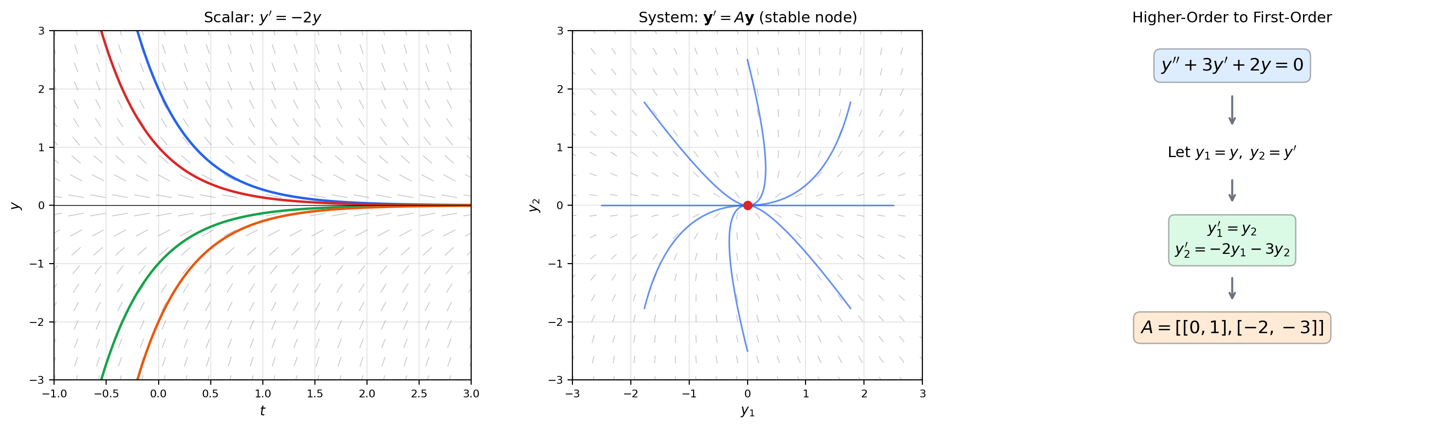
📝 Example 2 (Higher-order to first-order conversion)
The second-order equation converts to a first-order system via , :
Every -th order linear ODE becomes an first-order system. This reduction is not just a notational convenience — it places all linear ODEs (regardless of order) into a single framework where eigenvalue methods apply uniformly.
💡 Remark 1 (Autonomous vs. non-autonomous systems)
When is constant, the system is autonomous: the velocity field depends only on the state , not on time. This is the typical case in ML — the loss landscape does not change during training (for fixed data). Time-dependent systems are harder and appear in §7 via the non-homogeneous formulation.
2. The Matrix Exponential
The scalar ODE has the solution . The system has the solution , where the matrix exponential is defined by the power series:
This series always converges for any square matrix and any . The proof uses the submultiplicativity of the operator norm: , so the series is dominated by .
The matrix exponential is a power series in the matrix variable , with infinite radius of convergence. Everything we proved about scalar power series in Topic 18 — absolute convergence, term-by-term differentiation — extends to matrix-valued series.
📐 Definition 2 (Matrix Exponential)
For any matrix and scalar , the matrix exponential is
where (the identity matrix) and denotes the -th matrix power. The series converges absolutely in any matrix norm.
🔷 Theorem 1 (Convergence of the Matrix Exponential)
For any and , the series converges absolutely, and .
Proof.
For any submultiplicative norm , we have
The scalar series converges (it is the exponential function evaluated at ). Therefore the matrix series converges absolutely by comparison.
Absolute convergence in a finite-dimensional normed space implies convergence (because with any matrix norm is a complete normed space), so is well-defined.
The bound follows from the triangle inequality applied to the partial sums:
🔷 Theorem 2 (Properties of the Matrix Exponential)
Let and . Then:
(a) .
(b) .
(c) for all .
(d) is invertible with .
(e) If , then .
(f) If , then in general.
💡 Remark 2 (The commutativity caveat)
Property (e) fails without commutativity. The Baker-Campbell-Hausdorff formula gives the correction: where is the commutator. This non-commutativity is why matrix exponentials are harder than scalar exponentials, and why Lie theory is the natural language for matrix groups. In ML, this matters when composing transformations that don’t commute — rotation followed by scaling is not the same as scaling followed by rotation.
📝 Example 3 (Diagonal and nilpotent exponentials)
If , then — each component evolves independently.
If is nilpotent ( for some ), then — a matrix polynomial in , since all higher powers vanish. This finite truncation makes nilpotent exponentials easy to compute.

3. Eigenvalue Methods — Diagonalizable Systems
If has linearly independent eigenvectors — i.e., is diagonalizable with where — then the matrix exponential factors cleanly:
This reduces the system to independent scalar equations. The general solution is , where are the eigenvectors and are determined by the initial condition. Each term is a scalar ODE solution (Topic 21) dressed in the direction of its eigenvector.
The Jacobian introduced eigendecomposition as a change of basis that diagonalizes a linear map. Here the same idea solves a differential equation: in the eigenbasis, the coupled system decouples into independent exponentials.
🔷 Theorem 3 (Solution via Eigendecomposition)
Let be diagonalizable with eigenvalues and corresponding linearly independent eigenvectors . The general solution of is
where (or ) are constants determined by .
Proof.
Each satisfies
because . By linearity of differentiation, any linear combination is also a solution.
Since is a basis for , every initial condition can be uniquely represented, so the general solution captures all solutions.
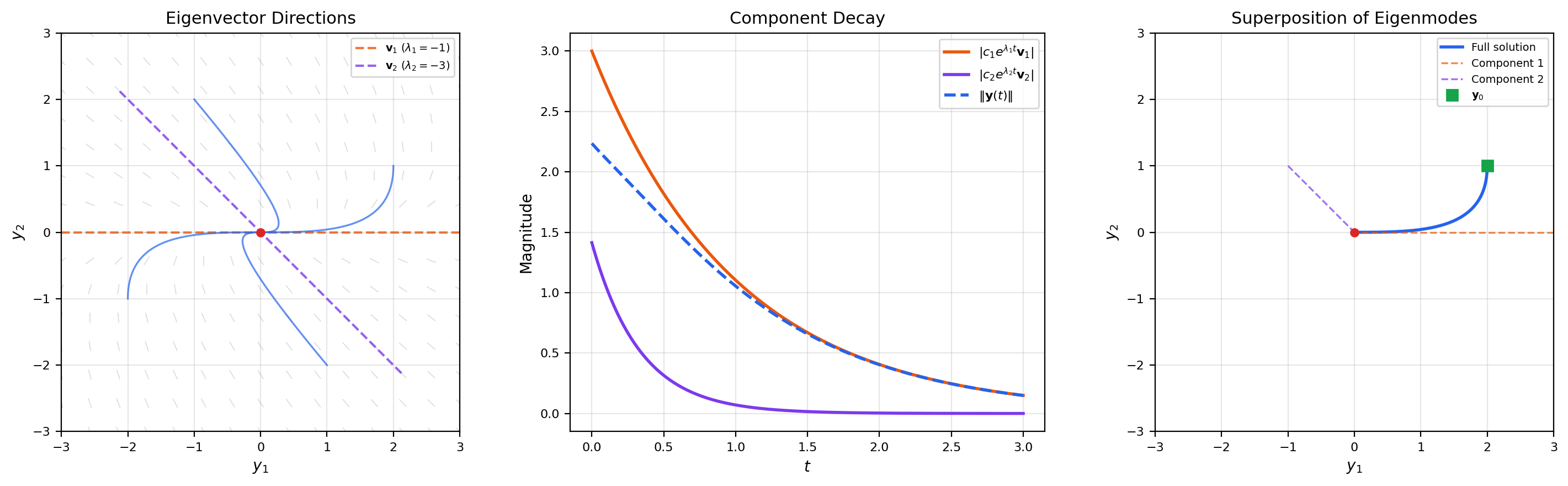
📝 Example 4 (A 2×2 system with real eigenvalues)
Consider . The eigenvalues are , , with eigenvectors , . The general solution is
Both eigenvalues are negative, so all solutions decay to the origin — a stable node. The fast component () dies out first, and trajectories ultimately align with the slow eigendirection .
📝 Example 5 (Complex eigenvalues)
The rotation matrix has eigenvalues . The solution is — pure rotation in the phase plane (a center). With damping, (), the eigenvalues become , and solutions spiral inward — a stable spiral.
💡 Remark 3 (Real solutions from complex eigenvalues)
When is real and is a complex eigenvalue with eigenvector , the two real-valued solutions are
The factor controls growth or decay; and produce rotation. When , we get spirals that decay inward; when , spirals that grow outward; when , closed ellipses.
4. Phase Portraits for 2×2 Systems
For a system , the qualitative behavior is completely determined by the eigenvalues of . The trace-determinant plane organizes all possibilities into a single diagram — one of the most useful classification tools in dynamical systems.
The eigenvalues of a matrix are , where and . Every qualitative feature of the phase portrait — stability, oscillation, node vs. spiral — is encoded in these two numbers.
📐 Definition 3 (Phase Portrait)
The phase portrait of is the collection of all solution trajectories plotted in the phase plane . The origin is the only equilibrium point (assuming is invertible, i.e., ).
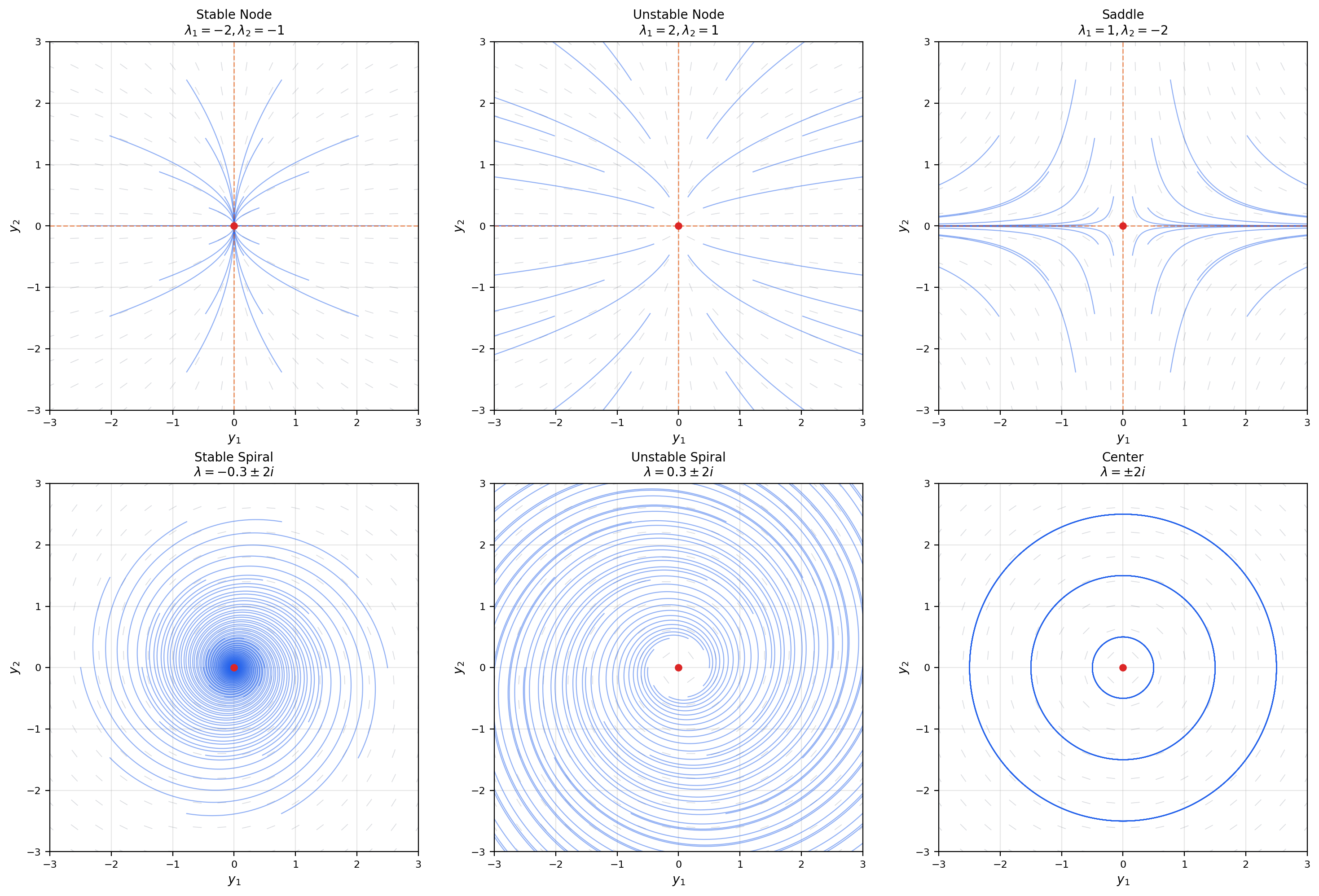
🔷 Theorem 4 (Trace-Determinant Classification)
Let be a real matrix with and , and define the discriminant . The phase portrait of is classified as follows:
(i) : saddle (eigenvalues of opposite sign).
(ii) , , : stable node (distinct negative real eigenvalues).
(iii) , , : unstable node (distinct positive real eigenvalues).
(iv) , , : stable spiral (complex eigenvalues with negative real part).
(v) , , : unstable spiral (complex eigenvalues with positive real part).
(vi) , : center (pure imaginary eigenvalues).
(vii) : degenerate (at least one zero eigenvalue; line of equilibria).
📝 Example 6 (The trace-determinant plane as a map)
Place a dot at for any matrix, and the diagram immediately tells you the phase portrait type. The parabola separates nodes from spirals. The -axis () separates stable from unstable. The -axis () separates saddles from non-saddles. Every linear system lives at exactly one point on this map.
💡 Remark 4 (Phase portraits and the Hessian)
Compare with the second-derivative test: the Hessian’s eigenvalues classify critical points of a function as minima (), maxima (), or saddle points (mixed signs). The ODE system matrix’s eigenvalues classify equilibria as stable nodes, unstable nodes, or saddles — the same eigenvalue analysis, governing dynamics instead of statics. Gradient descent connects them: near a critical point.
5. Repeated and Complex Eigenvalues — Beyond Diagonalizability
What happens when is defective — a repeated eigenvalue with only one linearly independent eigenvector? The matrix is not diagonalizable, and the Jordan normal form provides the solution. We find a generalized eigenvector satisfying (where is the eigenvector), and the solution involves terms — the same polynomial-times-exponential that appeared in the scalar repeated-root case.
📐 Definition 4 (Generalized Eigenvector)
A vector is a generalized eigenvector of rank 2 for with eigenvalue if , where is an eigenvector (, ). More generally, a generalized eigenvector of rank satisfies but .
🔷 Theorem 5 (Solution for Defective 2×2 Systems)
If has a repeated eigenvalue with a single eigenvector and generalized eigenvector (with ), then the general solution is
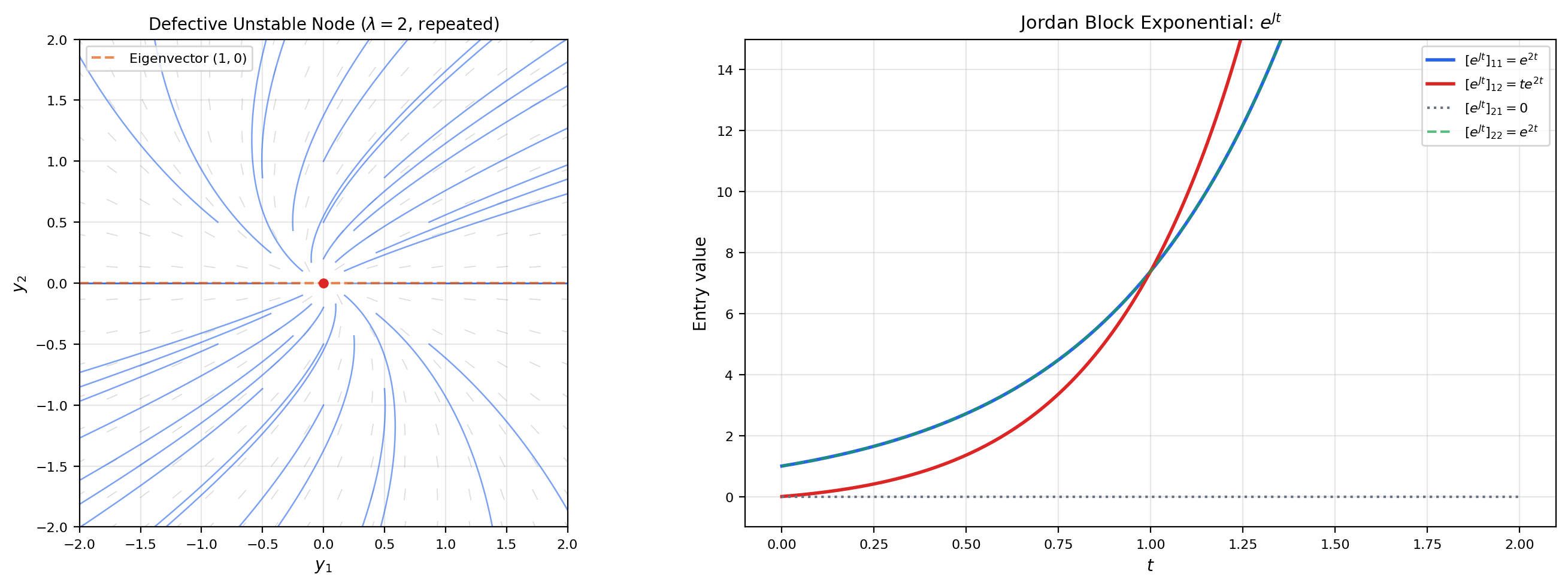
📝 Example 7 (A defective node)
. The repeated eigenvalue is , with a single eigenvector . The generalized eigenvector satisfies , giving . The solution is
The phase portrait is a degenerate unstable node — all trajectories are tangent to the eigenvector direction at the origin.
🔷 Proposition 1 (Jordan Normal Form and the Matrix Exponential)
If where is in Jordan normal form with blocks ( nilpotent), then where
This is a finite sum because is nilpotent ( for some ). Each Jordan block of size contributes terms for .
💡 Remark 5 (Defective matrices are rare but important)
Generically, matrices are diagonalizable — defective matrices form a set of measure zero in matrix space. But in applications, defective matrices arise naturally at bifurcation points — the boundary between qualitatively different behaviors. The transition from a stable spiral to a stable node passes through a defective node at on the trace-determinant diagram. Stability & Dynamical Systems will examine these transitions systematically.
6. Fundamental Matrices & the Wronskian
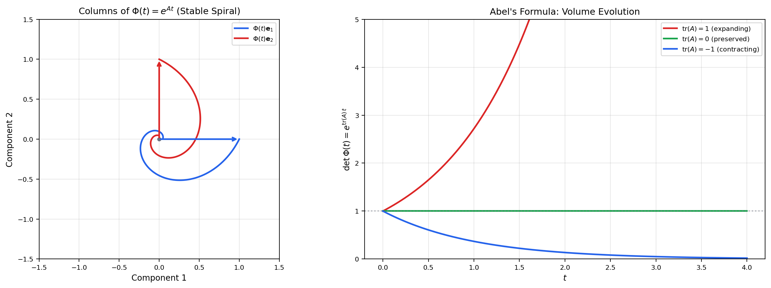
A fundamental matrix is an matrix whose columns are linearly independent solutions. For the system , the standard choice is , satisfying . Abel’s formula connects the determinant of the fundamental matrix (the Wronskian) to the trace of , telling us exactly how volumes evolve under the flow.
📐 Definition 5 (Fundamental Matrix)
A fundamental matrix for the system is a matrix-valued function satisfying whose columns are linearly independent solutions. The standard fundamental matrix is , satisfying .
🔷 Theorem 6 (Abel's Formula (Liouville's Formula))
If is a fundamental matrix for , then
For the standard fundamental matrix, .
Proof.
We show that — a scalar linear ODE with solution .
For the derivative of the determinant: by the multilinearity of the determinant in its rows,
where replaces the -th row of with its derivative (the -th row of ).
The -th row of is . By the alternating property of the determinant, a matrix with two identical rows has determinant zero. Therefore, only the diagonal term survives in each :
This is the scalar ODE with , whose unique solution is .
💡 Remark 6 (Volume evolution)
Abel’s formula says that the flow of preserves volume if and only if . Hamiltonian systems (from classical mechanics) have and are volume-preserving — this is Liouville’s theorem. Dissipative systems () contract volumes, which is why stable systems have trajectories that converge to lower-dimensional attractors.
7. Non-Homogeneous Systems & Variation of Parameters
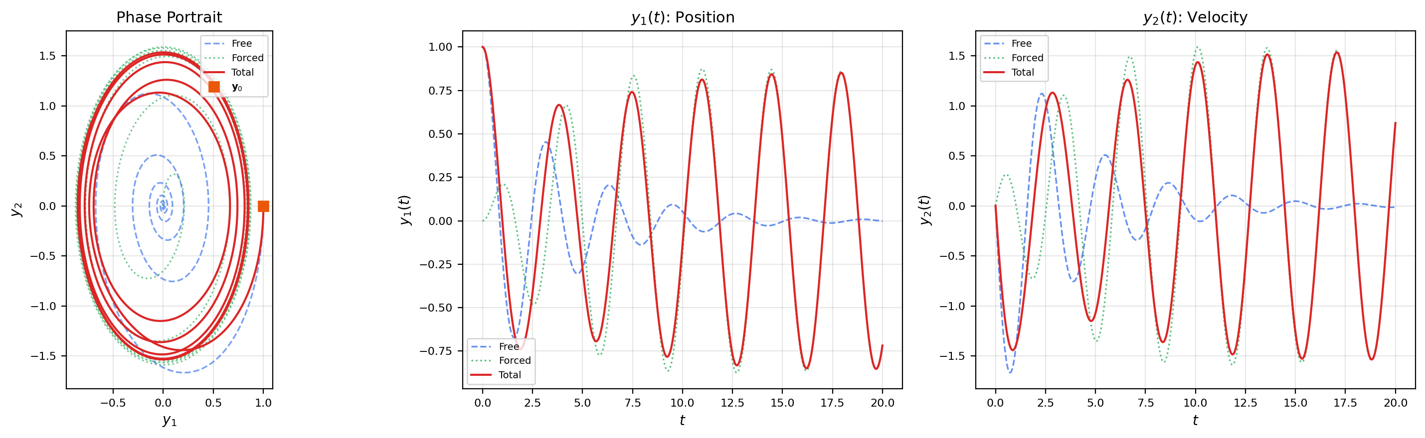
The non-homogeneous system adds a forcing term — an external input that drives the system. The solution method is variation of parameters: replace the constant vector in the homogeneous solution by a time-dependent vector , and solve for .
🔷 Theorem 7 (Variation of Parameters for Linear Systems)
The solution of the IVP , is:
The first term is the homogeneous solution (free response); the integral is the convolution of the matrix exponential with the forcing (forced response).
Proof.
Let (variation of parameters ansatz). Differentiating using the product rule:
Comparing with gives , so .
Integrating with the initial condition :
Substituting back: .
📝 Example 8 (Forced harmonic oscillator)
The system models a harmonic oscillator driven by an external force at frequency . The convolution integral produces resonance when — the forced response grows without bound because the driving frequency matches the natural frequency.
📝 Example 9 (Input-output systems and the transfer function)
Writing , (state-space form), the output is
The matrix is the impulse response — the system’s output when the input is a delta function. This is exactly the structure of state-space models in ML (S4/Mamba): the matrices , , are learned, and the matrix exponential mediates between continuous and discrete representations.
💡 Remark 7 (Convolution and the Laplace transform)
The variation of parameters formula is a matrix convolution. The Laplace transform converts this to an algebraic equation: . The transfer matrix encodes the system’s frequency response. The poles of the transfer function are the eigenvalues of — connecting back to the phase portrait classification.
8. Existence, Uniqueness & the Vector Picard-Lindelöf Theorem
The Picard-Lindelöf theorem (Topic 21) extends directly to vector-valued IVPs. For linear systems, the Lipschitz condition is automatically satisfied: , so the Lipschitz constant is simply . Moreover, linear systems never blow up in finite time — solutions exist for all .
🔷 Theorem 8 (Picard-Lindelöf for Vector IVPs)
Let be continuous on an open set and Lipschitz in :
Then the IVP , has a unique local solution.
🔷 Corollary 1 (Global Existence for Linear Systems)
If is constant and is continuous, then the IVP , has a unique solution on all of .
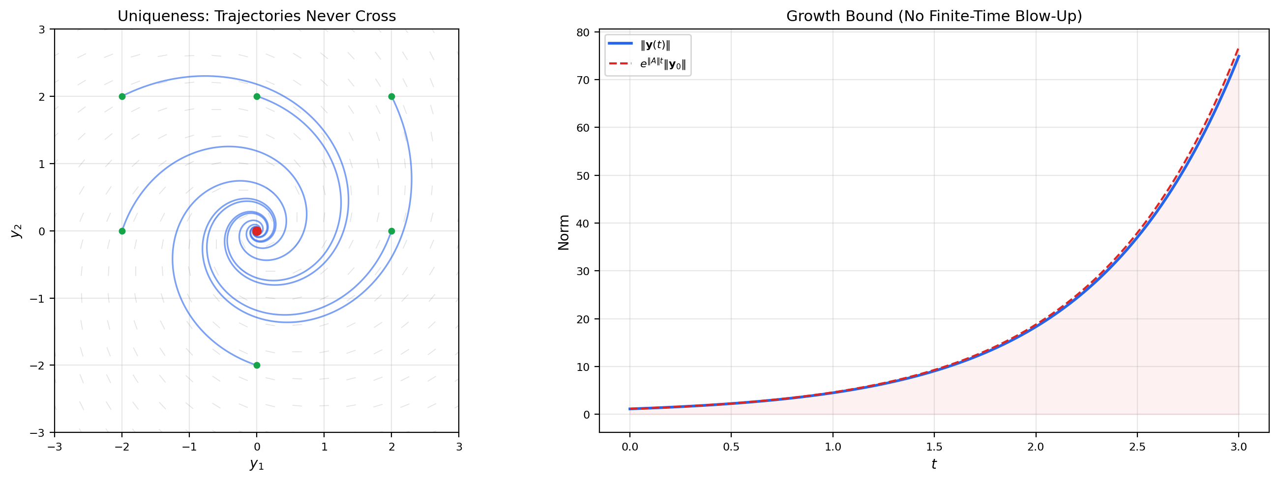
This follows because is globally Lipschitz with constant , and the Grönwall inequality prevents blow-up: .
💡 Remark 8 (Linear systems never blow up)
Compare with Topic 21’s blow-up example , where the nonlinearity causes finite-time escape to infinity. For linear systems, the solution grows at most exponentially: . Exponential growth is fast, but it never reaches infinity in finite time. This is why linearization is always locally valid — the linear approximation never predicts blow-up.
💡 Remark 9 (Uniqueness implies no trajectory crossing)
In the phase plane, solution trajectories of never cross (except at the origin, which is an equilibrium). If two trajectories crossed at a point at time , that point would have two distinct solutions to the same IVP — contradicting uniqueness. This topological consequence constrains the geometry of phase portraits: trajectories can approach or depart from the origin, but they cannot intersect.
9. ML Connections — State-Space Models, Training Dynamics, and Continuous-Time Architectures
Linear systems are not just a theoretical stepping stone — they are the mathematical backbone of several active research areas in machine learning. The matrix exponential, eigenvalue decomposition, and phase portrait analysis appear directly in the design and analysis of modern architectures.
9.1: Gradient descent as a linear system
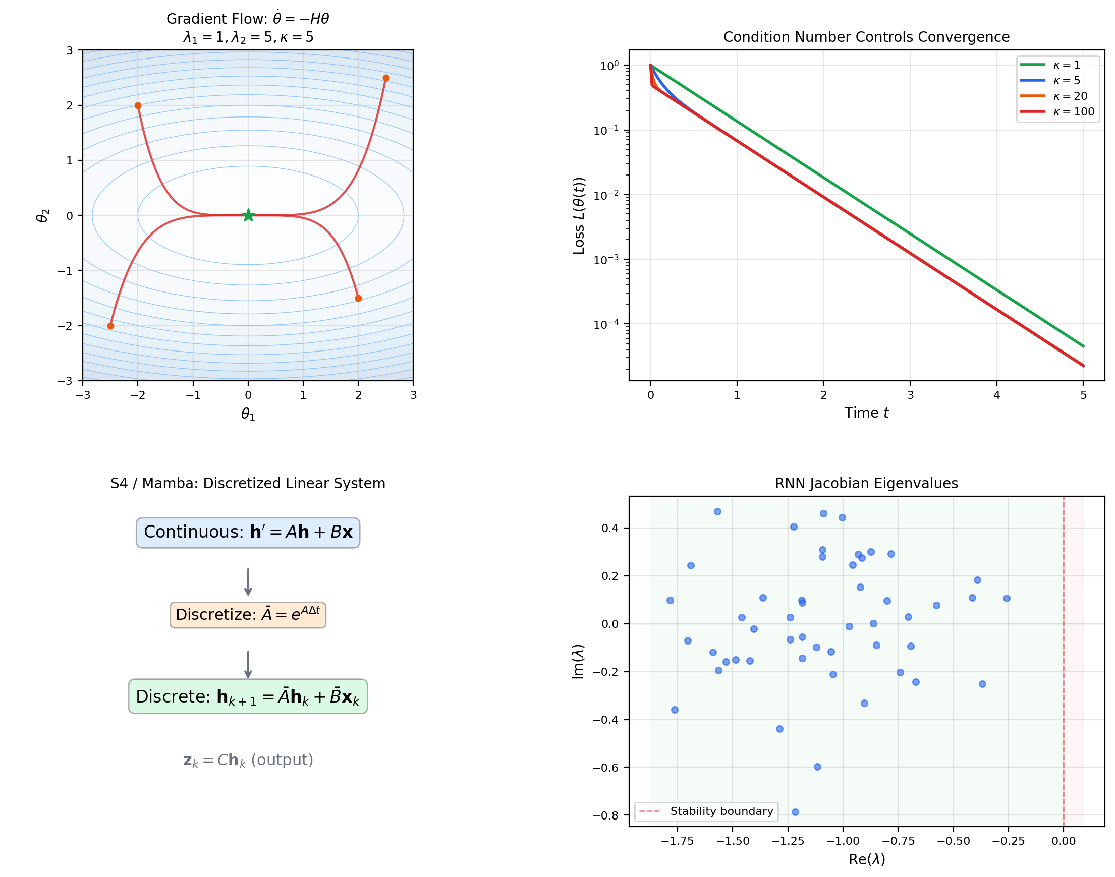
Near a critical point of a smooth loss , the gradient flow linearizes to where is the Hessian and . The solution decays along each eigendirection of at rate .
The slowest mode () dominates: convergence is governed by , and the condition number measures how anisotropic the convergence is. This is why preconditioning (replacing with , as in Newton’s method) speeds up training — it makes all eigenvalues equal, so all directions converge at the same rate.
📝 Example 10 (Quadratic loss and eigen-decomposition of convergence)
Consider with . The gradient flow has solution .
After time , the residual error in each direction is : direction 3 converges 100× faster than direction 1. The loss shows multi-scale decay — a fast initial drop (the large-eigenvalue components) followed by a long tail (the small-eigenvalue component).
9.2: Structured state-space models (S4/Mamba)
The S4 architecture (Gu et al. 2022) parameterizes a sequence model as a continuous-time linear system:
The matrices , , are learned parameters. The system is discretized for training: where — the matrix exponential from this topic.
📝 Example 11 (S4 discretization via matrix exponential)
Given continuous parameters , the discrete parameters are and (assuming is invertible). This exact discretization preserves the dynamics of the continuous system. The bilinear (Tustin) approximation is a Padé approximant that preserves stability — mapping eigenvalues with negative real part to eigenvalues inside the unit circle.
9.3: Continuous-time RNNs and neural CDEs
A continuous-time RNN replaces the discrete update with the ODE . Near a fixed point, this is a linear system whose dynamics are governed by the Jacobian . The eigenvalues of determine whether the hidden state remembers (eigenvalues near 0) or forgets (eigenvalues ) — the vanishing/exploding gradient problem in its continuous-time form.
9.4: Spectral analysis of training dynamics
The loss Hessian’s eigenvalue distribution controls training: the bulk spectrum determines the average learning speed, while outlier eigenvalues (from batch normalization, skip connections, or specific data directions) create fast modes that converge first. The matrix exponential encodes the full training dynamics: each eigen-component is an independent exponential decay, and the superposition of all components determines the loss trajectory. Understanding this spectral picture is the gateway to spectral methods in ML.
Connections & Further Reading
Prerequisites — topics you need first
First-Order ODEs & Existence Theorems
The scalar linear ODE y' + p(t)y = q(t) from Topic 21 is the 1×1 case of y' = Ay + g(t). The integrating factor e^{∫p(t)dt} becomes the matrix exponential e^{At}. The Picard-Lindelöf theorem extends to vector IVPs with the same proof — the Lipschitz constant is the operator norm ‖A‖.
The Jacobian & Multivariate Chain Rule
The matrix A in y' = Ay is the Jacobian of the right-hand side — constant, so the linearization is exact. The eigendecomposition A = PDP⁻¹ is a change of basis that diagonalizes the linear map, the same operation introduced in Topic 10 for understanding how the Jacobian distorts neighborhoods.
Power Series & Taylor Series
The matrix exponential e^{At} = Σ (At)^k/k! is a power series in the matrix variable At. Convergence is proved using the operator norm and the ratio test, exactly as for scalar power series in Topic 18. The radius of convergence is infinite — the matrix exponential converges for all t and all A.
The Hessian & Second-Order Analysis
Phase portrait classification by eigenvalues of A mirrors the second-derivative test from Topic 11: the Hessian's eigenvalues classify critical points as minima, maxima, or saddle points; the system matrix's eigenvalues classify equilibria as stable nodes, unstable nodes, or saddles.
The Derivative & Chain Rule
The matrix exponential satisfies d/dt[e^{At}] = Ae^{At}, the matrix analog of d/dt[e^{at}] = ae^{at}. The chain rule extends: d/dt[e^{f(t)A}] = f'(t)Ae^{f(t)A}.
Completeness & Compactness
Convergence of the matrix exponential series requires completeness of the normed space of n×n matrices. The argument parallels the scalar case (absolute convergence of Σ‖A‖^k t^k/k!) but takes place in a finite-dimensional Banach algebra.
Where this leads — next in formalCalculus
On to formalStatistics — where this calculus powers inference
On to formalML — where this calculus powers ML
Gradient Descent
Gradient descent on a quadratic loss L(θ) = ½θᵀHθ is the linear system θ̇ = −Hθ with solution θ(t) = e^{−Ht}θ₀. The eigenvalues of the Hessian H determine convergence rates: each eigen-component decays as e^{−λᵢt}. The condition number κ(H) = λ_max/λ_min is the ratio of fastest to slowest decay, explaining why ill-conditioned problems converge slowly.
Spectral Theorem
The spectral decomposition A = PDP⁻¹ is the computational engine of the matrix exponential. The spectral theorem guarantees that symmetric matrices have real eigenvalues and orthogonal eigenvectors, yielding e^{At} = Σ e^{λᵢt}vᵢvᵢᵀ — a sum of rank-one exponentials. This spectral representation appears in kernel methods (Mercer's theorem), PCA, and spectral graph theory.
Information Geometry
Natural gradient descent θ̇ = −F⁻¹∇L defines a linear system in the tangent space of the statistical manifold. The Fisher information matrix F acts as the metric tensor, and the matrix exponential e^{−F⁻¹∇²L·t} describes local training dynamics in natural gradient coordinates.
References
- book Arnold (1992). Ordinary Differential Equations Chapters 5–6 develop the matrix exponential and phase portrait classification from the geometric viewpoint. The primary reference for our visualization-first approach to 2×2 systems
- book Teschl (2012). Ordinary Differential Equations Chapter 3 provides the rigorous treatment of linear systems, fundamental matrices, and variation of parameters. Clear and free online
- book Hirsch, Smale & Devaney (2013). Differential Equations, Dynamical Systems, and an Introduction to Chaos Chapters 2–6 are the standard reference for phase portrait classification and the trace-determinant diagram. Excellent for building geometric intuition
- book Meyer (2000). Matrix Analysis and Applied Linear Algebra Chapter 10 covers the matrix exponential, Jordan normal form, and matrix functions with full rigor. The computational reference for matrix exponential properties
- paper Gu, Goel & Ré (2022). “Efficiently Modeling Long Sequences with Structured State Spaces” The S4 paper — introduces structured state-space models (SSMs) as discretized linear systems y' = Ay + Bu with learned matrices. The matrix exponential is central to the discretization and efficient computation via the HiPPO framework
- paper Gu & Dao (2023). “Mamba: Linear-Time Sequence Modeling with Selective State Spaces” Extends S4 with input-dependent (selective) state-space parameters, achieving transformer-competitive performance. The linear system structure y' = A(x)y + B(x)u connects linear systems theory to modern sequence modeling
- paper Moler & Van Loan (2003). “Nineteen Dubious Ways to Compute the Exponential of a Matrix, Twenty-Five Years Later” The classic survey of matrix exponential computation methods — eigendecomposition, Padé approximation, scaling-and-squaring, ODE solvers. Essential context for the computational notes section