The Hessian & Second-Order Analysis
Second-order partial derivatives, the Hessian matrix as the Jacobian of the gradient, critical point classification via eigenvalues, the second-order Taylor expansion, and Newton's method — the curvature machinery behind second-order optimization
Abstract. The Hessian matrix H_f(a) collects all second-order partial derivatives of a scalar-valued function f: ℝⁿ → ℝ into an n × n symmetric matrix. It is precisely the Jacobian of the gradient: H_f = J(∇f) — the first-order derivative of the first-order derivative. Where the gradient tells us which direction is uphill (first-order, slope), the Hessian tells us how the surface curves (second-order, curvature). The eigenvalues of the Hessian are the principal curvatures: all positive indicate a bowl (local minimum), all negative indicate a dome (local maximum), and mixed signs indicate a saddle point. The second-order Taylor expansion f(a+h) ≈ f(a) + ∇f(a)·h + ½ hᵀ H_f(a) h approximates the function by a paraboloid, and classifying critical points reduces to analyzing this quadratic form. Newton's method x_{k+1} = x_k - H_f(x_k)⁻¹ ∇f(x_k) exploits the Hessian to take curvature-corrected optimization steps, achieving quadratic convergence where gradient descent converges only linearly. In machine learning, the Hessian governs loss surface geometry: its condition number κ(H) = λ_max/λ_min determines how much gradient descent struggles with elongated valleys, its spectrum reveals whether critical points are minima or saddle points (in high-dimensional problems, saddle points dominate), and second-order methods — from Newton to L-BFGS to natural gradient — all use the Hessian or its approximations to improve convergence. The Hessian is the bridge between the first-order world (gradient descent) and the second-order world (curvature-aware optimization).
Overview & Motivation
Gradient descent moves “downhill” — in the direction of steepest descent, . But it ignores curvature. In a narrow valley of the loss landscape, the gradient points roughly across the valley rather than along it, causing the optimizer to zigzag back and forth between the valley walls. The gradient tells you which direction is steepest, but it says nothing about how the steepness changes as you move.
The Hessian captures this missing information. Where the gradient is a vector of first-order partial derivatives (slope in each direction), the Hessian is a matrix of second-order partial derivatives (how the slope changes in each direction). Its eigenvalues tell you how steeply the surface curves in each principal direction, and its eigenvectors tell you which directions those are. A narrow valley has one large eigenvalue (steep walls) and one small eigenvalue (gentle slope along the floor) — and the ratio between them, the condition number , quantifies exactly how much trouble gradient descent will have.
Second-order methods like Newton’s method use the Hessian to take smarter steps — correcting for curvature so the optimizer moves along the valley floor instead of bouncing between the walls. The price is computing (or approximating) an matrix of second derivatives, which is why most deep learning still uses first-order methods. But understanding the Hessian is essential for understanding why gradient descent behaves the way it does — and the Hessian is literally the Jacobian of the gradient: . Everything we built in Topics 9 and 10 converges here.
Second-Order Partial Derivatives & Clairaut’s Theorem
Partial derivatives are themselves functions, so we can differentiate them again. If has partial derivatives and , then is itself a function of , and we can take its partial derivative with respect to or . This gives us four second-order partial derivatives: , , , and .
📐 Definition 1 (Second-Order Partial Derivative)
Let have partial derivative in a neighborhood of . If is itself differentiable with respect to at , the second-order partial derivative is
When , this is the unmixed (or pure) second partial derivative . When , this is a mixed partial derivative.
Notation: , , .
The order in the notation matters: we differentiate first with respect to (innermost), then with respect to (outermost). This raises a natural question: does the order of differentiation matter? For mixed partials, is always equal to ?
🔷 Theorem 1 (Clairaut's Theorem (Symmetry of Mixed Partials))
Let and suppose the mixed partial derivatives and both exist and are continuous in a neighborhood of . Then
In short: if (all second partial derivatives exist and are continuous), the order of differentiation does not matter. This ensures the Hessian matrix is symmetric.
Proof.
We prove the case. Let with continuous mixed partials and near . Define the second-difference quotient:
Let . Then . By the Mean Value Theorem, there exists between and such that:
Applying the Mean Value Theorem again to , there exists between and such that:
By the same argument with the roles of and reversed — define and apply the MVT twice — we obtain:
for some between and , between and .
As , we have and . Since and are continuous at :
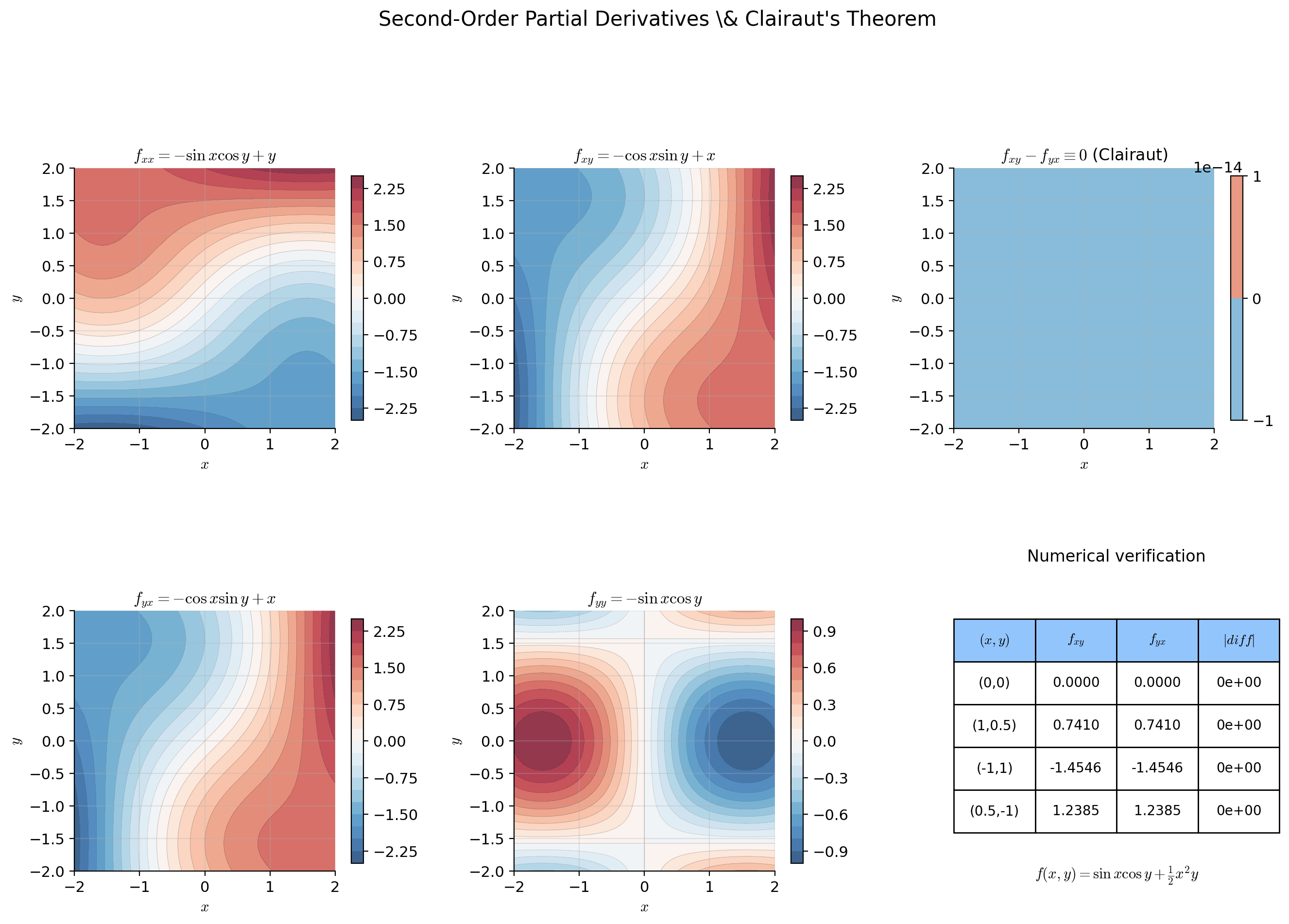
📝 Example 1 (Second-order partials of f(x,y) = x²y + sin(xy))
We compute all four second-order partial derivatives:
First partials:
Second partials:
Observe — Clairaut’s theorem confirmed. Both mixed partials are continuous, so the order of differentiation is interchangeable. The four second partials, assembled into a matrix, form the Hessian.
💡 Remark 1 (From second derivative to Hessian matrix)
In single-variable calculus (Topic 5), the second derivative is a single number. For , the second-order information consists of second partial derivatives. Clairaut’s theorem reduces this to independent values (the upper triangle of a symmetric matrix). For : 3 values (, , ). For (a small neural network): 5,050 values. For (a large language model): storing the full Hessian is infeasible — motivating the approximations discussed in Section 8.
The Hessian Matrix
📐 Definition 2 (The Hessian Matrix)
Let be twice differentiable at . The Hessian matrix of at is the matrix
If , then is symmetric by Clairaut’s theorem.
Notation: , , .
The key insight is that the Hessian is not a new concept — it is the Jacobian applied to the gradient.
🔷 Proposition 1 (Hessian is the Jacobian of the Gradient)
Let be . The gradient is a vector-valued function with component functions . Its Jacobian matrix is
Therefore . The Hessian is the Jacobian of the gradient. (The last equality uses the symmetry guaranteed by Clairaut’s theorem for functions — without symmetry, would be the transpose of the Hessian as defined above.)
Proof.
Direct verification. The -th component of is . By the definition of the Jacobian (Topic 10), the Jacobian of has entries:
By Clairaut’s theorem (Theorem 1), . Therefore .
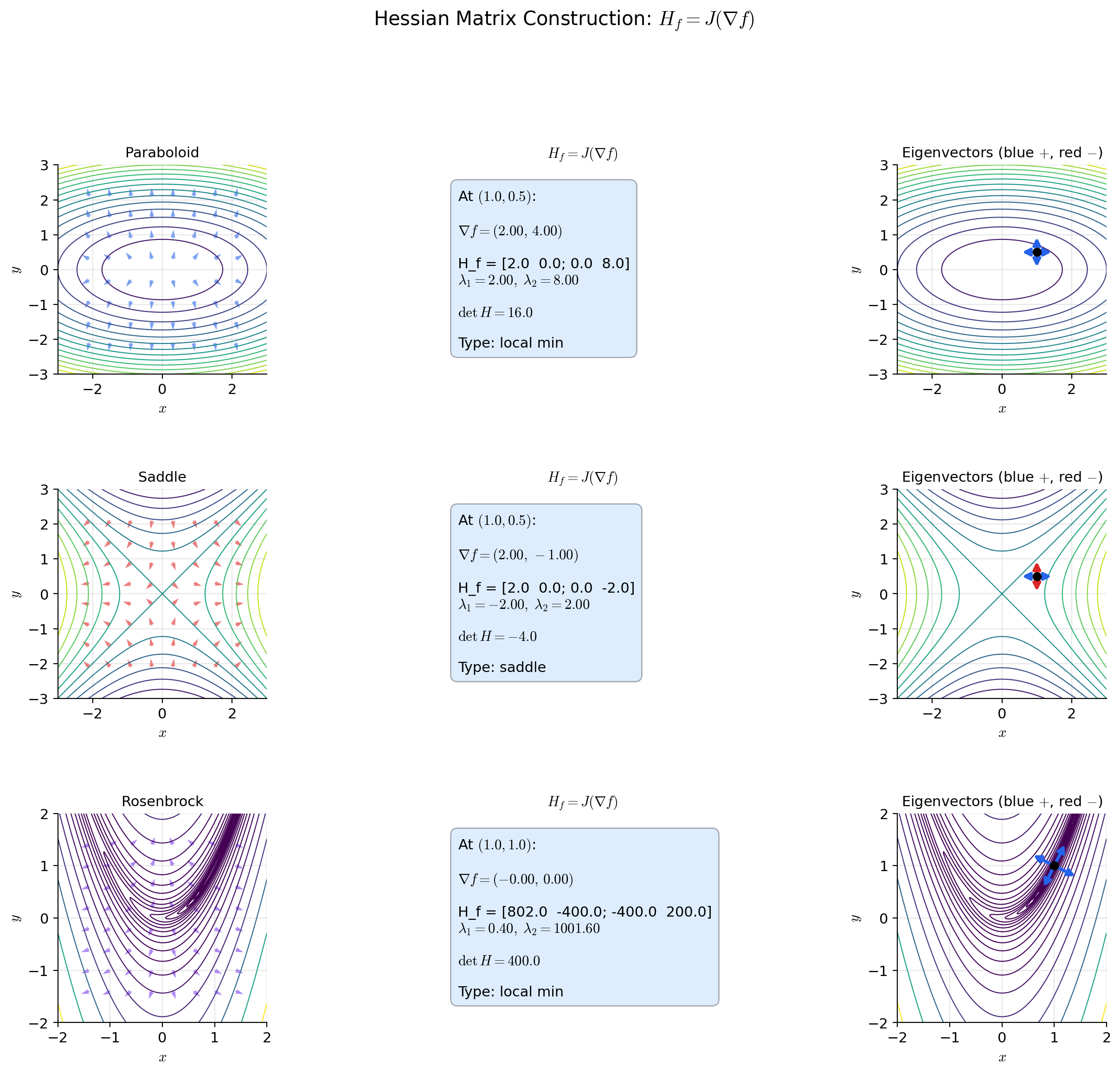
📝 Example 2 (Hessian of a paraboloid)
.
Gradient: .
Hessian:
— constant, independent of . The eigenvalues are 2 and 8. The surface curves 4 times more steeply in the -direction than in the -direction. This is the prototypical ill-conditioned loss surface: gradient descent zigzags because the curvatures are unequal. The condition number is .
📝 Example 3 (Hessian of a saddle function)
.
Gradient: .
Hessian:
One positive eigenvalue (2, curves upward in ) and one negative eigenvalue (, curves downward in ). The origin is a saddle point — a critical point that is neither a minimum nor a maximum. The surface looks like a horse saddle: it rises in one direction and descends in the other.
📝 Example 4 (Hessian of a neural network loss)
Consider a loss where is the sigmoid function. The Hessian has entries involving and — it depends on the data and the current parameters . Unlike the paraboloid, this Hessian is not constant — the curvature of the loss surface changes as the parameters move. Computing this matrix is cheap; computing a matrix for a real network is not. This is why practical deep learning relies on Hessian approximations rather than the full matrix.
Critical Point Classification
At a critical point where , the first-order Taylor term vanishes. The function near is governed by the second-order term:
The sign behavior of the quadratic form — does it produce all positive values, all negative values, or both? — determines whether is a local min, local max, or saddle. This is where eigenvalue analysis becomes essential.
📐 Definition 3 (Positive Definite, Negative Definite, Indefinite)
A symmetric matrix is:
- Positive definite () if for all . Equivalently, all eigenvalues of are positive.
- Negative definite () if for all . Equivalently, all eigenvalues are negative.
- Positive semidefinite () if for all . Equivalently, all eigenvalues are nonnegative.
- Negative semidefinite () if for all . Equivalently, all eigenvalues are nonpositive.
- Indefinite if takes both positive and negative values. Equivalently, has both positive and negative eigenvalues.
🔷 Proposition 2 (Eigenvalue Criterion for Definiteness)
Let be a symmetric matrix with eigenvalues . Then:
(a) .
(b) .
(c) is indefinite .
For : is positive definite iff and . It is indefinite iff .
📐 Definition 4 (Saddle Point)
A point is a saddle point of if and is indefinite — i.e., curves upward in some directions and downward in others. Near a saddle point, for some directions and for others. The origin of is the canonical example.
🔷 Theorem 2 (The Second Derivative Test (Multivariable))
Let be near , and suppose (so is a critical point). Then:
- If (positive definite), then is a strict local minimum.
- If (negative definite), then is a strict local maximum.
- If is indefinite, then is a saddle point.
- If is positive or negative semidefinite (has a zero eigenvalue), the test is inconclusive — higher-order analysis is needed.
For , write and let . Then:
- and : local minimum.
- and : local maximum.
- : saddle point.
- : inconclusive.
Proof.
We sketch the proof via the second-order Taylor expansion (proven in Section 5). At a critical point where :
Case 1: . By the spectral theorem for symmetric matrices, where is the smallest eigenvalue. For sufficiently small, the error is dominated by , so for all in a neighborhood — is a strict local minimum.
Case 2: . Analogous, with all inequalities reversed.
Case 3: indefinite. Let be an eigenvector with positive eigenvalue and an eigenvector with negative eigenvalue . Along for small : . Along : . So is neither a local min nor a local max — it is a saddle point.
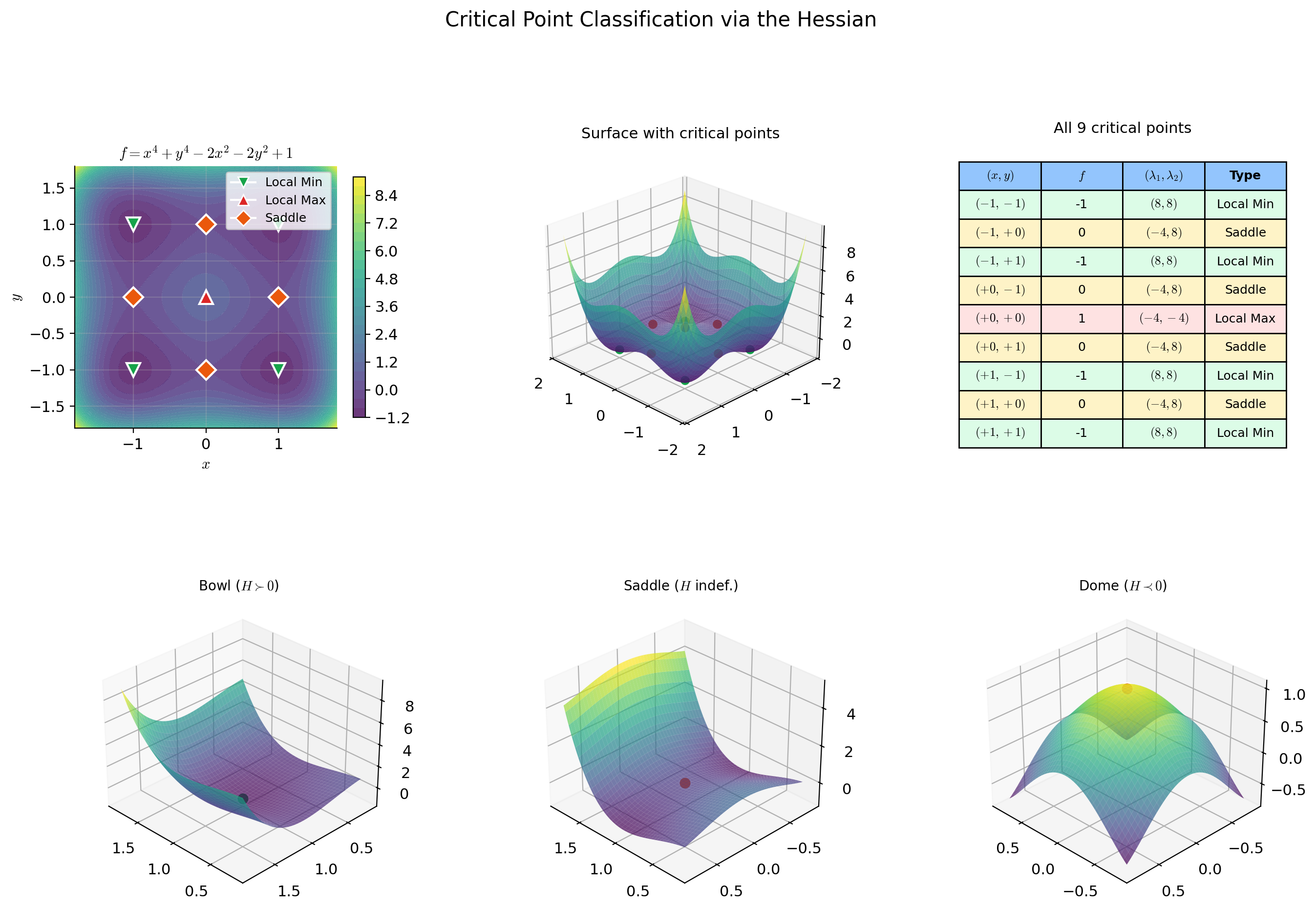
📝 Example 5 (Critical point classification: f(x,y) = x⁴ + y⁴ − 2x² − 2y² + 1)
Gradient: . Setting both components to zero: and . The critical points are all combinations of and — nine points total.
Hessian:
At : — local maximum.
At : — indefinite — saddle point. Similarly for , , .
At : — local minimum. Similarly for , , .
Nine critical points: 1 local max, 4 saddle points, 4 local minima.
💡 Remark 2 (When the second derivative test is inconclusive)
The function has and — the zero matrix. The test is inconclusive. Yet the origin is clearly a local (and global) minimum: for all .
The issue is that the second-order Taylor expansion is not informative when the quadratic term vanishes — the fourth-order terms dominate. Compare with : same zero Hessian at the origin, but now the origin is a saddle point (of fourth order). The zero Hessian tells us the second-order analysis has nothing to say — we need higher-order derivatives to classify the point.
The Second-Order Taylor Expansion
Just as the first-order Taylor expansion approximates by a hyperplane (the tangent plane from Topic 9), the second-order expansion approximates by a paraboloid. The Hessian provides the curvature information that the gradient approximation misses.
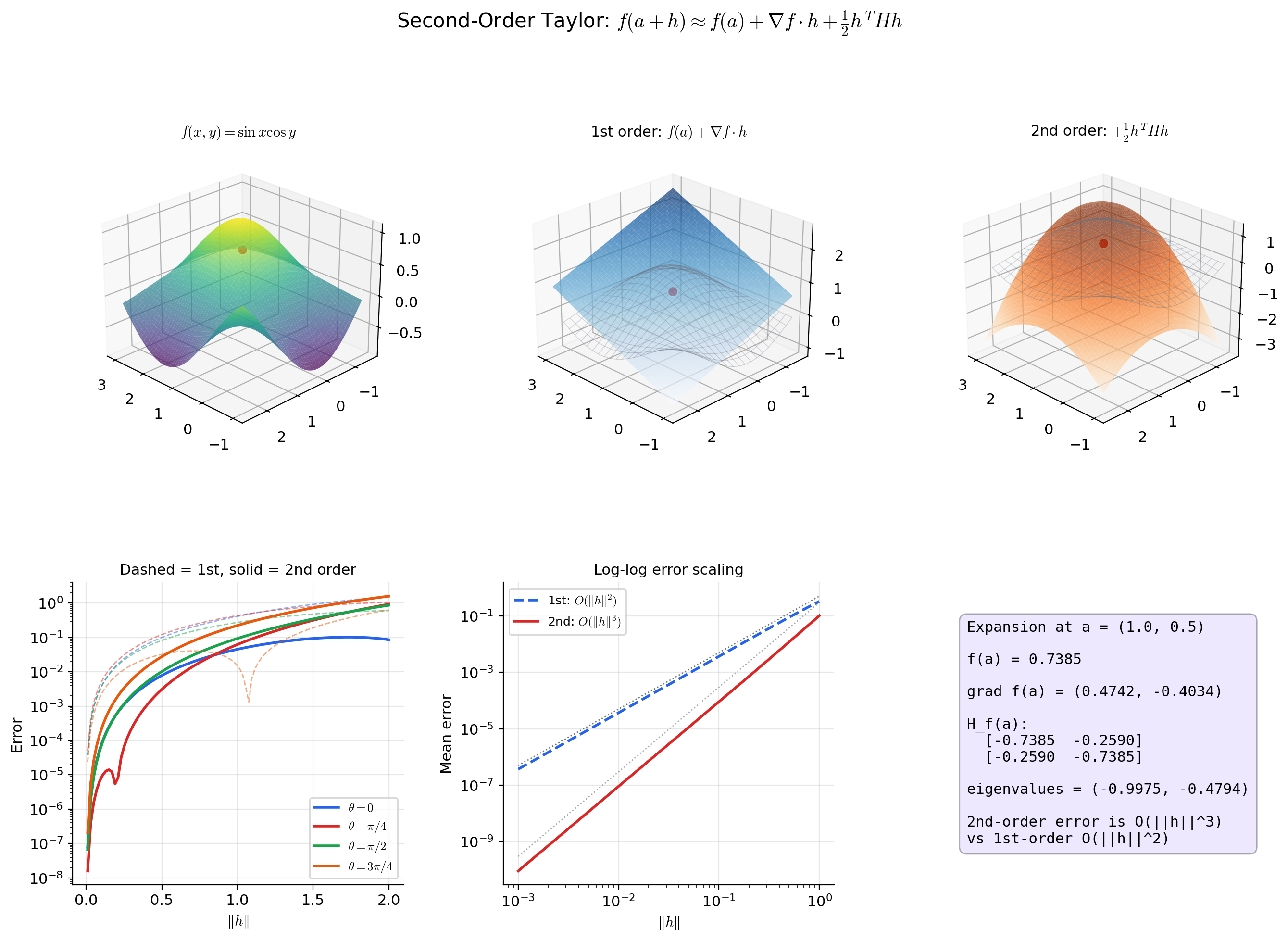
🔷 Theorem 3 (Second-Order Taylor Expansion)
Let be in a neighborhood of . Then for all with in that neighborhood:
where the remainder satisfies , i.e., .
In expanded form:
This is the multivariable generalization of from Topic 6.
Proof.
Apply the single-variable Taylor expansion to the function at :
We compute the derivatives of :
- .
- by the chain rule. So .
- . So .
Setting :
The error bound conversion from at to uses the continuity of the second partial derivatives.
📝 Example 6 (Quadratic approximation of f(x,y) = eˣ⁺ʸ near the origin)
At : , , .
The second-order Taylor expansion:
This matches the known Taylor series with . The Hessian captures the curvature of at the origin: it curves equally in all directions within the subspace and is flat in the perpendicular direction — reflected by the eigenvalues 0 and 2.
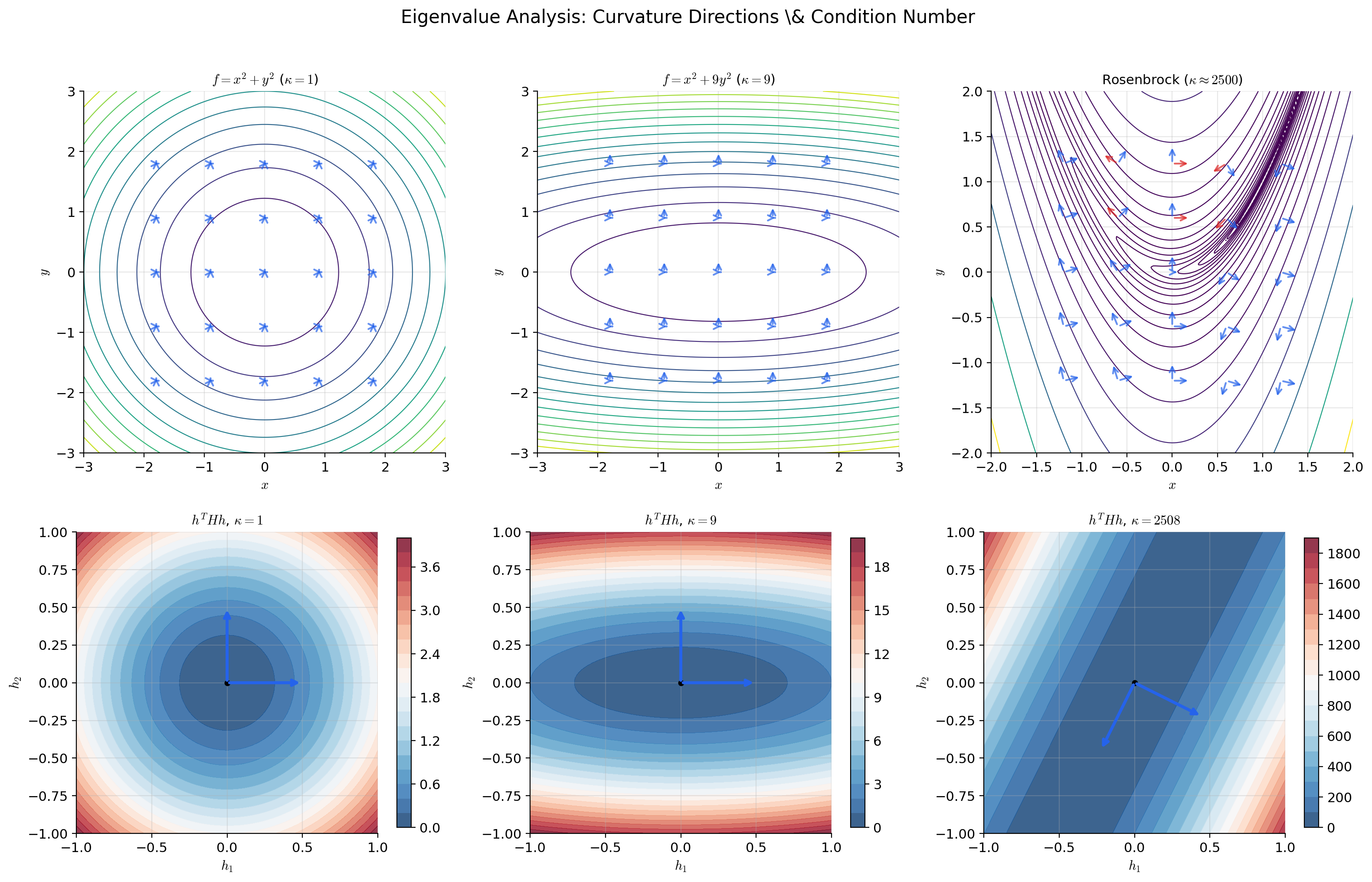
Eigenvalue Analysis & Curvature
The eigenvalues and eigenvectors of have direct geometric meaning. The eigenvalues are the principal curvatures — the maximum and minimum curvatures of at . The eigenvectors are the principal curvature directions. This section connects the algebraic classification (Definition 3) to geometric visualization.
📝 Example 7 (Curvature of the elliptic paraboloid)
For with :
Eigenvalues: , , with eigenvectors along the coordinate axes. The condition number measures eccentricity.
When : (circular contours, isotropic curvature — gradient descent converges in a straight line).
When or : (elliptical contours, anisotropic curvature — gradient descent zigzags). The severity of the zigzag is directly proportional to .
📝 Example 8 (The monkey saddle: f(x,y) = x³ − 3xy²)
Gradient: , so is a critical point.
Hessian at origin:
The second derivative test is inconclusive. Yet the surface has three “valleys” meeting at the origin (picture a monkey sitting with both legs and a tail hanging down). This is a degenerate critical point requiring third-order analysis — the Hessian’s silence here tells us that the curvature is zero in all directions, so the second-order Taylor expansion provides no useful local information.
💡 Remark 3 (The condition number and optimization)
For a quadratic with , gradient descent with optimal step size converges in iterations, where is the condition number. Newton’s method converges in iterations (quadratic convergence).
The gap is dramatic: for , gradient descent needs roughly 7,000 steps while Newton needs roughly 10. The condition number at a local minimum of a non-quadratic loss measures the local version of this problem — it tells you how much the loss landscape stretches gradient descent steps in the worst direction relative to the best.
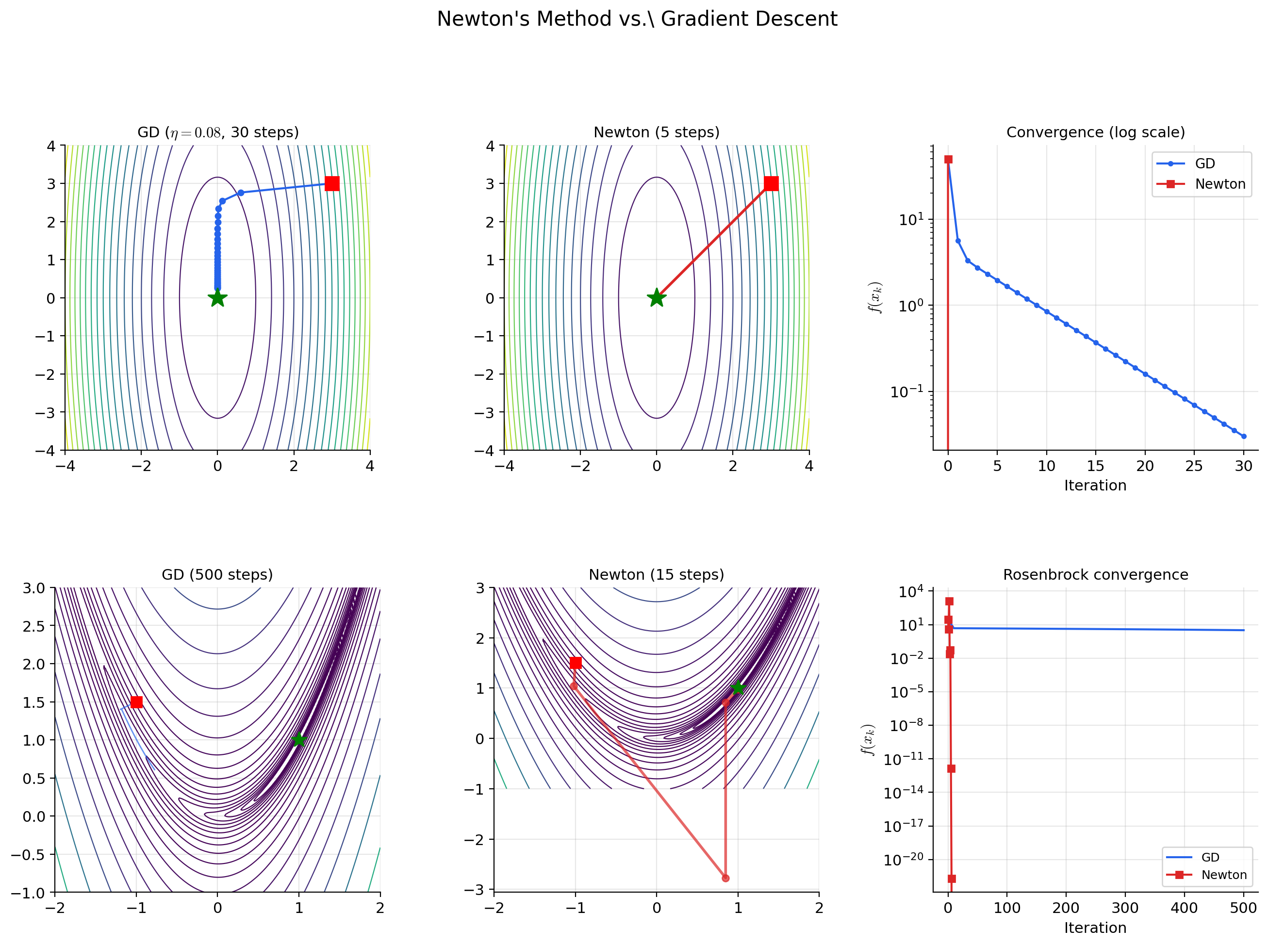
Newton’s Method
Newton’s method uses the quadratic approximation from the second-order Taylor expansion to take curvature-corrected steps. At each iterate, we approximate by a paraboloid, find the minimum of the paraboloid (which has a closed-form solution), and move there.
📝 Example 9 (Newton's method derivation)
At the current iterate , approximate by its second-order Taylor expansion:
This is a quadratic function of . Its gradient with respect to is , which vanishes when:
The Newton update is:
Compare with gradient descent: . Newton replaces the scalar step size with the matrix — a direction- and curvature-dependent step that accounts for the local shape of the surface.
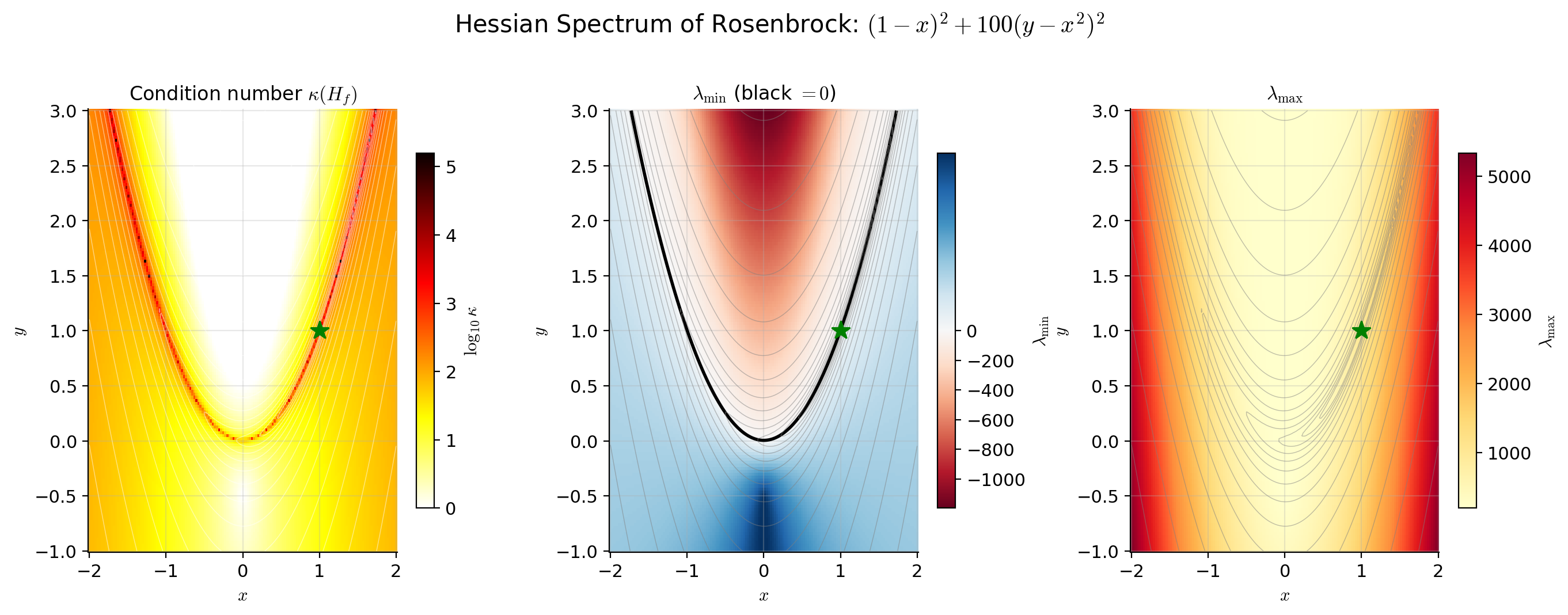
📝 Example 10 (Newton on the Rosenbrock function)
.
The minimum is at . Gradient descent converges slowly because the loss landscape is a narrow, curved valley with condition number at the minimum. The gradient points nearly perpendicular to the valley floor, so GD bounces between the walls with each step.
Newton’s method converges in a few iterations because it uses the Hessian to navigate the curvature. The Hessian-inverse premultiplication rotates the gradient to align with the valley floor and scales the step to match the local curvature — exactly the correction that gradient descent is missing.
💡 Remark 4 (Newton's method can fail)
Newton’s method requires to be positive definite — otherwise the quadratic model has no minimum (it has a maximum or saddle). At a saddle point, is indefinite, and the Newton step may move toward the saddle rather than away from it.
This is why second-order methods in practice often use modified Newton methods that ensure the step direction is always a descent direction. Common modifications include:
- Levenberg-Marquardt damping: Replace with for some , shifting all eigenvalues to be positive.
- Trust region methods: Constrain and solve the constrained quadratic subproblem.
- Eigenvalue modification: Replace negative eigenvalues with their absolute values before inverting.
Connections to Statistics
The Hessian is the central object of Fisher information, asymptotic variance of the MLE, the curvature of penalized objectives, and the Laplace approximation. Wherever uncertainty quantification or second-order optimization shows up in statistics, the Hessian is doing the work.
Fisher information
Expected Fisher information and observed information are Hessians of the negative log-likelihood. The asymptotic variance of the MLE is . Positive-definiteness of governs identifiability and curvature. See formalStatistics Maximum Likelihood.
Laplace approximation and BIC
. The determinant of the Hessian at the MAP is the volume correction; BIC is the asymptotic form of this expansion. See formalStatistics Bayesian Model Comparison & BMA.
GLMs and penalized convexity
The GLM information matrix is a Hessian. Ridge adds to the Hessian, strictly improving conditioning; convexity of the penalized objective is a positive-semidefinite-Hessian condition. See formalStatistics Generalized Linear Models and formalStatistics Regularization & Penalized Estimation.
Information criteria
TIC replaces the AIC penalty with where and are observed/expected Fisher information — both Hessians. BIC’s asymptotic derivation uses the log-determinant of the Hessian at the MLE. See formalStatistics Model Selection & Information Criteria.
Connections to ML
Loss surface curvature
The Hessian of the loss function at the current parameters determines how the loss surface curves. The eigenvalues of are the curvatures in each principal direction. A large condition number means the surface is an elongated valley — gradient descent overshoots in steep directions and barely moves in flat directions.
This is why learning rate tuning is difficult: no single scalar works well for all directions simultaneously. If is small enough not to overshoot in the steepest direction, it makes negligible progress in the flattest direction. If is large enough to make progress in the flat direction, it oscillates wildly in the steep direction.
Batch normalization, layer normalization, and careful weight initialization schemes all implicitly improve the Hessian’s condition number by making the loss surface more isotropic — reducing the gap between the largest and smallest curvatures.
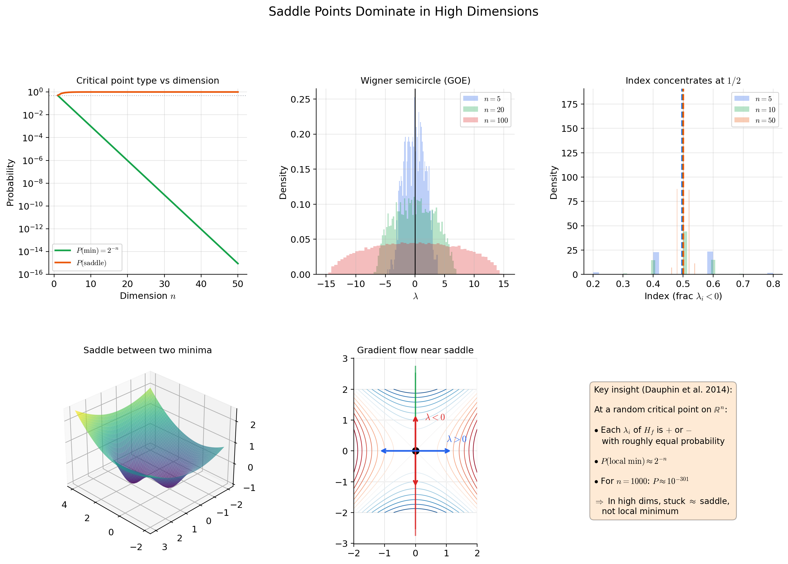
Saddle points in high dimensions
Dauphin et al. (2014) showed that in high-dimensional optimization, saddle points are exponentially more common than local minima. At a random critical point of a generic function on , each eigenvalue of the Hessian is independently positive or negative with roughly equal probability.
A local minimum requires all eigenvalues to be positive — probability roughly . A saddle point (mixed eigenvalue signs) has probability roughly . For : the probability of a random critical point being a local minimum is approximately .
The practical implication: when gradient descent appears to “get stuck” in high-dimensional optimization, it is almost certainly near a saddle point, not a local minimum. Gradient descent can escape saddle points (slowly, along directions of negative curvature), but Newton’s method can actually be attracted to saddle points (because amplifies components along eigenvectors with small eigenvalues, which near saddle points includes directions with negative curvature).
Second-order optimizers
-
Full Newton: . Quadratic convergence but memory and computation per step. Impractical for .
-
Quasi-Newton (L-BFGS): Approximates from gradient differences across recent steps — stores where – is the memory parameter. Widely used in scientific computing and small-scale ML.
-
Hessian-free optimization: Uses conjugate gradient to solve without forming explicitly — only requires Hessian-vector products , which can be computed via automatic differentiation in time (one forward + one backward pass per product).
-
Natural gradient: where is the Fisher information matrix. This is Newton’s method on the KL divergence rather than the loss — it adapts the step to the geometry of the probability distribution. See Information Geometry on formalML.
-
Adam and diagonal approximations: Adam’s per-parameter adaptive learning rate implicitly approximates the diagonal of . The second-moment estimate tracks the mean square of gradients, which under stationary conditions approximates the diagonal Fisher information.
Hessian spectrum in practice
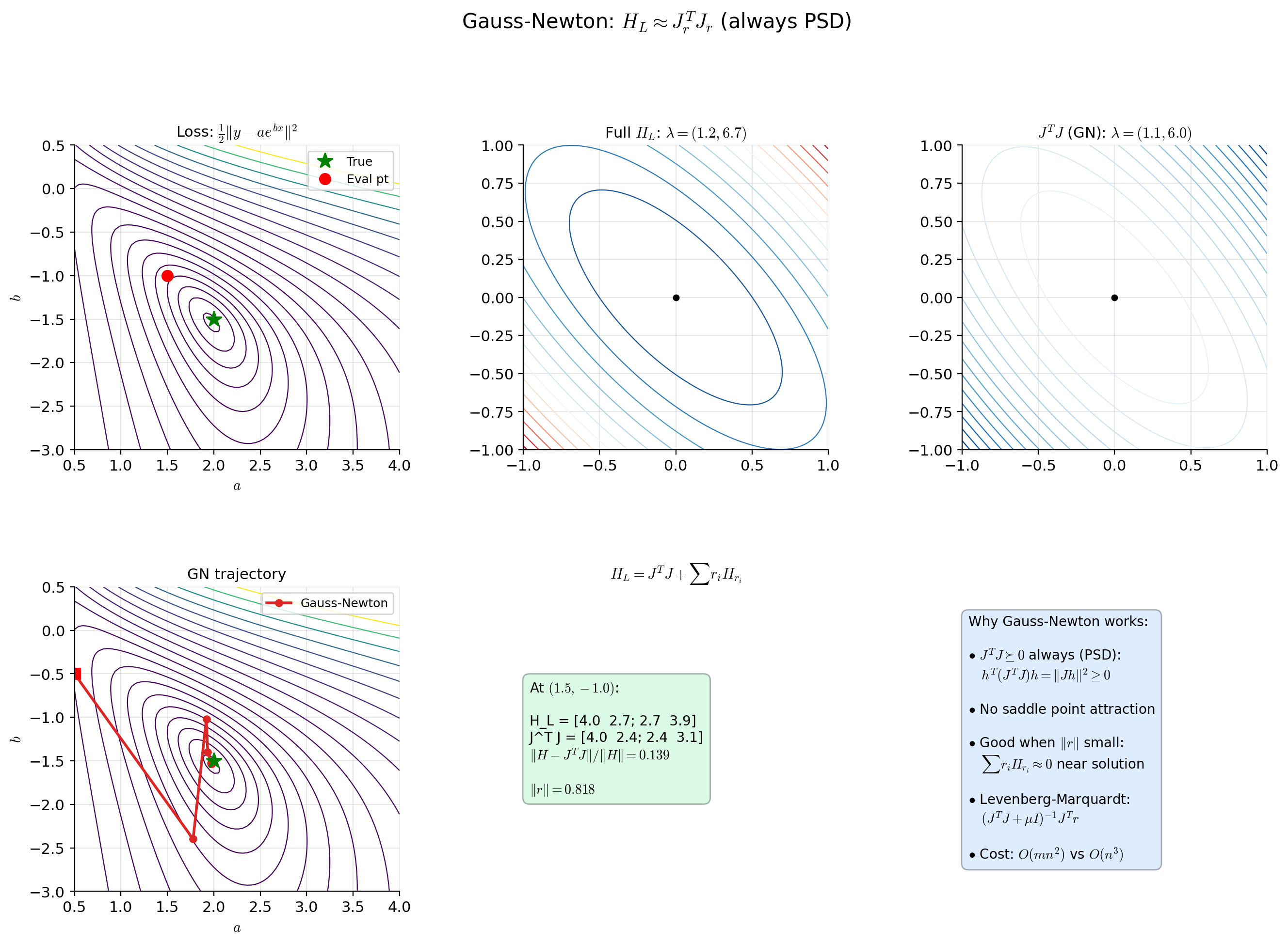
Empirical studies of neural network loss surfaces show that the Hessian spectrum is highly structured: most eigenvalues are near zero (flat directions corresponding to redundant parameters), a few are large and positive (high-curvature directions), and at saddle points, a few are negative. The “effective dimension” of the optimization problem is much smaller than , which explains why first-order methods work surprisingly well despite the theoretical superiority of second-order methods.
The Gauss-Newton approximation (where is the Jacobian of the residuals) is always positive semidefinite and provides a useful approximation to the Hessian for least-squares problems, avoiding the indefiniteness issue of the full Hessian.
Connections & Further Reading
Prerequisites — topics you need first
The Jacobian & Multivariate Chain Rule
The Hessian is the Jacobian of the gradient: H_f(a) = J(∇f)(a). This is the foundational identity — it says the Hessian is not a new concept but the Jacobian machinery from Topic 10 applied to the specific vector-valued function ∇f. The chain rule from Topic 10 also enables the second-order chain rule for composed functions.
Partial Derivatives & the Gradient
The gradient ∇f(a) from Topic 9 provides the first-order information (slope). The Hessian provides the second-order information (curvature). At a critical point where ∇f(a) = 0, the gradient vanishes and the Hessian takes over — it determines whether the critical point is a minimum, maximum, or saddle.
The Derivative & Chain Rule
The single-variable second derivative f''(a) from Topic 5 is the 1 × 1 case of the Hessian. The second derivative test (f''(a) > 0 → local min, f''(a) < 0 → local max) generalizes to the eigenvalue criterion: positive definite Hessian → local min, negative definite → local max.
Mean Value Theorem & Taylor Expansion
Taylor's theorem from Topic 6 provides the single-variable version of the second-order expansion f(a+h) = f(a) + f'(a)h + ½f''(a)h² + O(h³). The multivariable second-order Taylor expansion in this topic replaces f''(a)h² with the quadratic form h^T H_f(a) h.
Where this leads — next in formalCalculus
Inverse & Implicit Function Theorems
The Hessian analyzes the local structure of constraint surfaces near critical points — the inverse and implicit function theorems handle the regularity conditions under which those surfaces are smooth manifolds where second-order analysis applies.
Stability & Dynamical Systems
Eigenvalue analysis of the Hessian of a Lyapunov function determines equilibrium stability — the same curvature machinery used to classify optimization critical points classifies equilibria of dynamical systems.
Eigenvalues & Eigenvectors
On to formalStatistics — where this calculus powers inference
Maximum Likelihood
Expected Fisher information I(θ) = -E[∇²_θ log L] and observed information J(θ̂) = -∇²_θ log L(θ̂) are Hessians of the negative log-likelihood. The asymptotic variance of the MLE is I(θ_0)⁻¹. Positive-definiteness of I governs identifiability and curvature.
Bayesian Model Comparison And Bma
Laplace approximation: ∫ exp(ℓ(θ)) dθ ≈ exp(ℓ(θ̂)) · (2π)^(d/2) · |det(-∇²ℓ(θ̂))|^(-1/2). The determinant of the Hessian at the MAP is the volume correction; BIC -2·ℓ(θ̂) + d·log(n) is the asymptotic form of this expansion.
Generalized Linear Models
The GLM information matrix H(β) = -X^T W(β) X is a Hessian. Newton-Raphson / IRLS uses this to compute the update step. Positive-definiteness (from positive W diagonal entries) gives local convexity of the negative log-likelihood.
Regularization And Penalized Estimation
Convexity of the penalized objective L(β) + λ P(β) is a positive-semidefinite-Hessian condition. Ridge adds λI to the Hessian, strictly improving conditioning. Lasso's subdifferential structure replaces the Hessian at non-smooth points.
Model Selection And Information Criteria
TIC (Takeuchi IC) replaces the AIC penalty 2d with tr(J · I⁻¹) where J, I are observed/expected Fisher information — both Hessians. BIC's asymptotic derivation uses the log-determinant of the Hessian at the MLE.
Linear Regression
Topic 21's §21.7 characterizes the hat matrix H = X(X^T X)⁻¹X^T as a symmetric idempotent projector with eigenvalues in {0, 1} — exactly the spectral fact about symmetric matrices the Hessian topic develops. §21.8 Proof 9's Cochran theorem on quadratic forms in Normal vectors splits sums-of-squares into independent χ² components via the same eigenstructure.
On to formalML — where this calculus powers ML
Gradient Descent
Second-order optimization methods (Newton, quasi-Newton, L-BFGS) use the Hessian to precondition gradient descent. The condition number κ(H_f) = λ_max/λ_min determines the convergence rate — gradient descent takes O(κ) iterations, while Newton's method converges quadratically. Adaptive optimizers like Adam implicitly approximate diagonal Hessian elements.
Convex Analysis
A C² function f is convex if and only if H_f(x) ⪰ 0 for all x. Strong convexity (H_f ⪰ μI) provides the convergence rate guarantee μ/L for gradient descent, where L is the Lipschitz constant of the gradient (equivalently, the largest eigenvalue of the Hessian).
Information Geometry
The Fisher information matrix I(θ) equals the expected Hessian of the negative log-likelihood E[-H_{log p(x|θ)}] under regularity conditions. The natural gradient I(θ)⁻¹ ∇L(θ) is Newton's method adapted to the Riemannian geometry of the statistical manifold — the curvature here is the Hessian of the KL divergence.
Variational Bayes For Model Selection
§3's Laplace approximation evaluates the negative Hessian of $\log p(x, \theta)$ at the MAP as the posterior precision matrix; the determinant of that Hessian appears in the Laplace volume element and produces the BIC penalty when $n$ grows. The relationship between Hessian curvature and Bayesian-evidence concentration is the geometric content of §3.
References
- book Munkres (1991). Analysis on Manifolds Chapter 3 develops higher-order derivatives and the second-order Taylor formula in ℝⁿ
- book Spivak (1965). Calculus on Manifolds Chapter 2 treats higher derivatives and the Taylor expansion for multilinear maps
- book Rudin (1976). Principles of Mathematical Analysis Chapter 9 on second-order differentiation — Theorem 9.41 is Clairaut's theorem on symmetry of mixed partials
- book Nocedal & Wright (2006). Numerical Optimization Chapters 2–3 on Newton's method, quasi-Newton methods, and the role of the Hessian in optimization convergence theory
- book Boyd & Vandenberghe (2004). Convex Optimization Chapter 9 on Newton's method for unconstrained optimization — convergence analysis via the Hessian's condition number
- book Goodfellow, Bengio & Courville (2016). Deep Learning Section 8.2 on challenges in optimization including saddle points, ill-conditioning, and the role of the Hessian spectrum
- paper Dauphin, Pascanu, Gulcehre, Cho, Ganguli & Bengio (2014). “Identifying and Attacking the Saddle Point Problem in High-Dimensional Non-Convex Optimization” Shows that in high-dimensional optimization, saddle points dominate local minima — the Hessian spectrum at critical points has a mixture of positive and negative eigenvalues with high probability
- paper Kingma & Ba (2015). “Adam: A Method for Stochastic Optimization” The Adam optimizer's per-parameter learning rates implicitly approximate diagonal Hessian elements via second-moment estimates