Completeness & Compactness
The structural properties of ℝ that guarantee limits exist and optima are attained — why regularization works and when your optimization problem has a solution
Abstract. The completeness of ℝ — every nonempty set bounded above has a least upper bound — is the axiom that separates the real numbers from the rationals and makes calculus possible. This single property implies the Monotone Convergence Theorem, the Bolzano-Weierstrass Theorem, and the Cauchy completeness that guarantees iterative algorithms converge to something. Compactness, the other structural pillar, says that a set K ⊆ ℝ is compact (closed and bounded) if and only if every sequence in K has a subsequence converging to a point in K (Heine-Borel). Compactness is the topological property behind the Extreme Value Theorem: continuous functions on compact sets attain their maximum and minimum, which is exactly the existence guarantee for optimization problems like min_{θ ∈ Θ} L(θ) when Θ is compact. In machine learning, neural network parameter spaces are ℝ^d — decidedly not compact. Regularization techniques (L2 weight decay constraining ‖θ‖₂ ≤ R, L1 lasso constraining ‖θ‖₁ ≤ R, gradient clipping, spectral normalization) effectively restrict parameters to compact subsets, restoring the existence guarantees that compactness provides. Coercive loss functions (L(θ) → ∞ as ‖θ‖ → ∞) offer an alternative: their sublevel sets are compact, so minimizers exist even on unbounded domains.
Overview & Motivation
Suppose you’re training a neural network and the loss decreases at every step: . This is a bounded, decreasing sequence of real numbers. Does it converge? And does there actually exist a parameter vector that achieves the infimum of the loss? The first question is about completeness; the second is about compactness. These are the two structural properties of that make calculus — and optimization — work.
In Sequences, Limits & Convergence, we used completeness when we proved the Monotone Convergence Theorem and the Bolzano-Weierstrass Theorem. In Epsilon-Delta & Continuity, we used compactness (implicitly) when we proved the Extreme Value Theorem and the Heine-Cantor Theorem. Now we develop the theory explicitly. We will see that a single axiom — the least upper bound property — is the foundation for all of these results, and that compactness is the structural property that makes continuous optimization well-posed.
This is where the abstraction level increases. In the first two topics, we worked with individual sequences and functions. Here we reason about structural properties of the real line itself — asking not “does this particular sequence converge?” but “what property of guarantees that every bounded monotone sequence converges?”
Completeness of ℝ — The Least Upper Bound Property
Why is not enough
Consider the set . This set is nonempty () and bounded above ( is an upper bound). Does have a least upper bound in ? If it did, that least upper bound would have to be — but . The rationals have a “hole” right where the supremum should be.
This is not an isolated curiosity. The rationals are riddled with such holes — one for every irrational number. A number system with holes cannot support calculus: limits might not exist, monotone sequences might not converge, and continuous functions might not attain their extrema. The real numbers are constructed precisely to fill these holes.
📐 Definition 1 (Upper Bound and Supremum)
Let be nonempty. A number is an upper bound of if for all . The supremum (least upper bound) is an upper bound of with the property that if is any other upper bound of , then .
Dually, is a lower bound of if for all , and the infimum is the greatest lower bound.
The supremum has a crucial characterization: is the unique number such that (i) is an upper bound of , and (ii) for every , there exists with . This “approximation property” — you can always find elements of arbitrarily close to — is what makes the supremum useful for proofs.
🔷 Theorem (Axiom — Completeness of ℝ (LUB Property))
Every nonempty subset of that is bounded above has a supremum in .
This is not a theorem we prove — it is the axiom that defines the real numbers. Every construction of (Dedekind cuts, Cauchy sequence completion of ) is designed to make this axiom true. And from this single axiom, the entire structure of calculus follows.
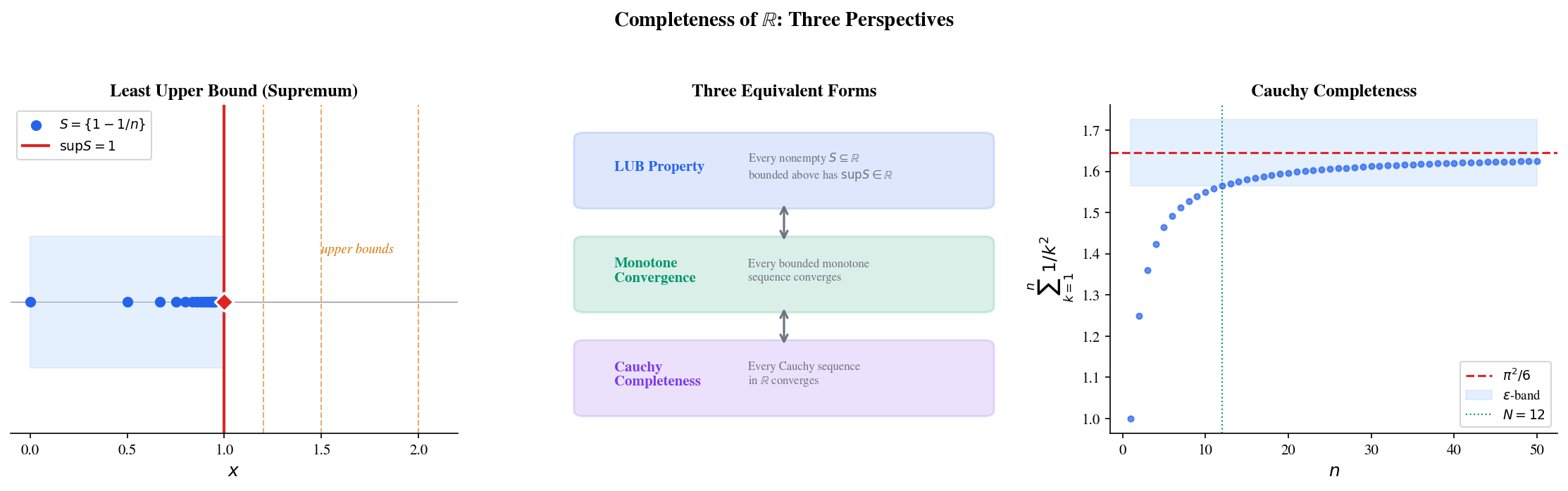
🔷 Theorem 1 (Equivalence of Completeness Formulations)
The following are equivalent:
(a) The LUB Property: Every nonempty subset of bounded above has a supremum in .
(b) Monotone Convergence Theorem: Every bounded monotone sequence in converges.
(c) Nested Interval Property: If is a nested sequence of closed bounded intervals with , then contains exactly one point.
(d) Cauchy Completeness: Every Cauchy sequence in converges to a point in .
Proof.
We sketch the cycle of implications.
(a) ⟹ (b): Let be bounded and increasing. The set is bounded above, so exists by the LUB property. For every , the approximation property gives for some . Since is increasing, for all . And since is an upper bound. So for all . This was proved as Theorem 1 in Sequences, Limits & Convergence.
(b) ⟹ (c): The sequence is increasing and bounded above (by ), so by MCT. Similarly is decreasing and bounded below. Since for all , we have . If , then , and .
(c) ⟹ Bolzano-Weierstrass: Given a bounded sequence in , repeatedly bisect: at least one half contains infinitely many terms. The Nested Interval Property guarantees the bisected intervals converge to a point, which is the limit of the extracted subsequence. This was the strategy behind Theorem 4 in Sequences, Limits & Convergence.
Bolzano-Weierstrass ⟹ (d): Every Cauchy sequence is bounded (proved in Sequences, Limits & Convergence, Theorem 5). Bolzano-Weierstrass gives a convergent subsequence . A Cauchy sequence with a convergent subsequence converges to the same limit: for , choose so that for and for . Then .
(d) ⟹ (a): Let be nonempty and bounded above. We construct a Cauchy sequence converging to . Start with any upper bound and any . Bisect : if the midpoint is an upper bound of , take the left half; otherwise, the right half. This produces intervals of width , and the endpoints form Cauchy sequences. By Cauchy completeness, they converge to some , which we verify is .
💡 Remark 1
In machine learning, completeness ensures that iterative algorithms have a limit. When gradient descent produces a Cauchy sequence of parameters — meaning the updates get arbitrarily small — completeness guarantees convergence to some . Without completeness, the “limit” might not exist, like in .
The Nested Interval Property
The equivalence theorem tells us the Nested Interval Property follows from completeness. But the NIP deserves a standalone treatment because it is the key proof technique for many existence theorems — and it is the theoretical backbone of bisection algorithms.
🔷 Theorem 2 (Nested Interval Property)
If is a nested sequence of closed, bounded intervals, then . If additionally , then the intersection contains exactly one point.
Proof.
Let , which exists by the LUB property since the are bounded above by . Let , which exists since the are bounded below by .
We claim . For any , the nesting gives (if , then ; if , then ). So every is an upper bound for , hence for all , hence .
Now for all (because and ), so .
If , then , so and the intersection is .
💡 Remark 2
The Nested Interval Property is the theoretical backbone of bisection-based algorithms. Every time you halve a search interval and keep the half containing your target, you are applying the NIP. Binary search, the bisection root-finding method from Epsilon-Delta & Continuity, and branch-and-bound optimization algorithms are all NIP in action. The visualization above lets you see this convergence directly — watch the interval width shrink exponentially while the endpoints close in on the target.
Open and Closed Sets
Before defining compactness, we need precise vocabulary for the topology of . The distinction between open and closed sets is not just a formality — it determines whether limits of sequences “stay inside” a set, which is exactly the property that makes compactness work.
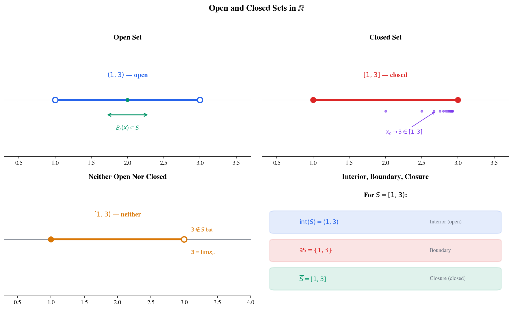
📐 Definition 2 (Open Set)
A set is open if for every , there exists such that the open ball . In other words, every point of has a “buffer zone” of neighboring points that also belong to .
📐 Definition 3 (Closed Set)
A set is closed if its complement is open. Equivalently, is closed if and only if it contains all its limit points: whenever is a sequence in with , then .
The sequential characterization is often more useful: a closed set is one that “keeps its limits.”
🔷 Proposition 1 (Properties of Open and Closed Sets)
(a) Arbitrary unions of open sets are open.
(b) Finite intersections of open sets are open.
(c) Arbitrary intersections of closed sets are closed.
(d) Finite unions of closed sets are closed.
Proof.
(a): If , then for some . Since is open, there exists with .
(b): If , then for each , there exists with . Take (this is where finiteness is essential — an infinite minimum of positive numbers could be zero). Then .
(c)–(d): Follow from (a)–(b) by De Morgan’s laws: and .
📐 Definition 4 (Interior, Boundary, Closure)
For :
- The interior is the largest open set contained in : the set of all for which some .
- The closure is the smallest closed set containing : equivalently, together with all its limit points.
- The boundary : the set of points where every neighborhood meets both and .
📝 Example 1
For :
- — the point has no neighborhood contained in (every contains negative numbers not in ).
- — the point is a limit point of (the sequence ) but .
- .
The set is neither open (0 is a boundary point in with no interior buffer) nor closed (1 is a limit point not in ).
Sequential Compactness
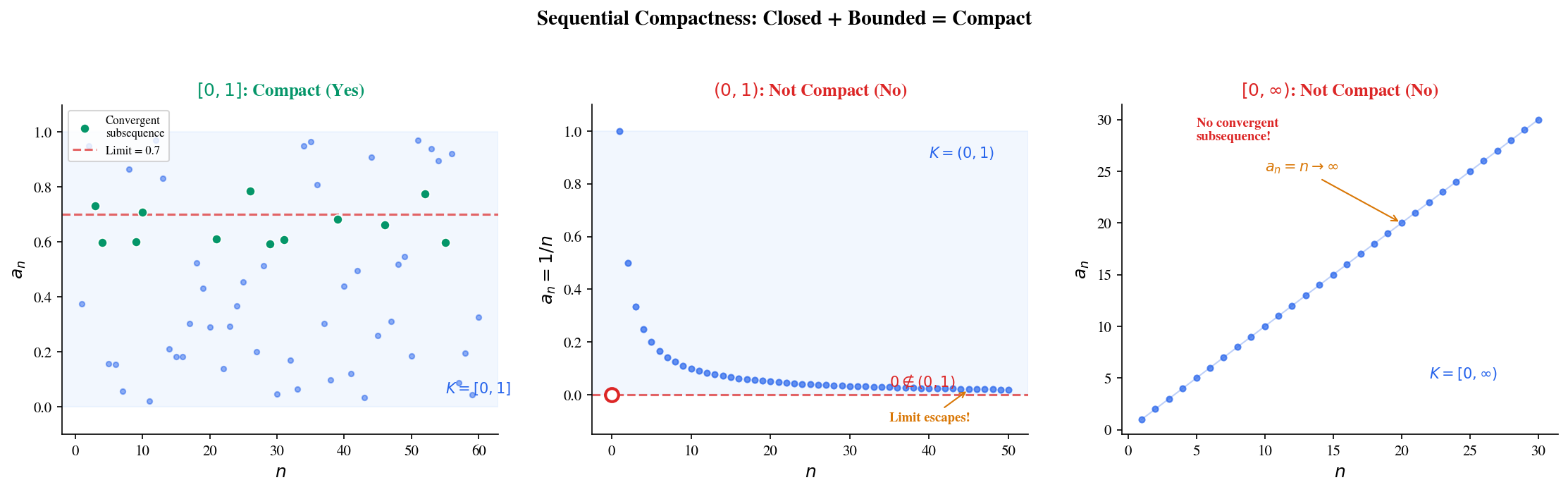
The Bolzano-Weierstrass Theorem from Sequences, Limits & Convergence says every bounded sequence in has a convergent subsequence. But where does that subsequence converge to? If the original sequence lives in , the limit is guaranteed to also be in — because is closed. If the sequence lives in , the limit might escape to 0 or 1. This is the difference between compact and non-compact.
📐 Definition 5 (Sequential Compactness)
A set is sequentially compact if every sequence in has a subsequence that converges to a point .
The key requirement is that the limit belongs to — not just that a convergent subsequence exists, but that the subsequence converges to a point inside the set.
🔷 Proposition 2 (Compact ⟺ Closed + Bounded in ℝ)
A subset is sequentially compact if and only if is closed and bounded.
Proof.
(⟸) Closed + bounded implies compact: If is bounded, then for some . By the Bolzano-Weierstrass Theorem, any sequence in has a convergent subsequence . If is closed, then (closed sets contain their limit points). So is sequentially compact.
(⟹) Compact implies closed: Suppose is not closed. Then there exists a sequence in with and . Every subsequence of also converges to (a fact from Sequences, Limits & Convergence). Since , no subsequence converges to a point in — contradicting sequential compactness.
(⟹) Compact implies bounded: Suppose is unbounded. Then for each , there exists with . The sequence has , so no subsequence can converge (convergent sequences are bounded). This contradicts sequential compactness.
💡 Remark 3
The characterization “closed + bounded ⟺ compact” is specific to — this is the Heine-Borel theorem we prove in the next section. In general metric spaces, compactness is a strictly stronger property than “closed + bounded.” For example, in the space of continuous functions with the supremum norm, the closed unit ball is closed and bounded but not compact — you can find a sequence of functions in it with no convergent subsequence. This distinction matters when working with function spaces in ML, and we develop it in Metric Spaces & Topology, where we prove that the sequence has all pairwise sup-norm distances , so no subsequence is Cauchy and no subsequence converges uniformly.
Compactness — The Open Cover Definition
Sequential compactness is intuitive: “every sequence has a convergent subsequence staying in the set.” There is an equivalent definition using open covers that is more powerful for proofs, especially when we generalize beyond .
📐 Definition 6 (Open Cover)
An open cover of is a collection of open sets such that . That is, every point of belongs to at least one of the .
A subcover is a subcollection that still covers . A finite subcover is a subcover with finitely many sets.
📐 Definition 7 (Compactness via Open Covers)
A set is compact if every open cover of has a finite subcover: for any collection of open sets covering , there exist finitely many such that .
🔷 Theorem 3 (Heine-Borel Theorem)
A subset is compact (every open cover has a finite subcover) if and only if is closed and bounded.
In , this means the compact sets are precisely the closed, bounded intervals and their closed subsets.
Proof.
We prove the theorem for ; the case follows by the same argument applied coordinate-wise.
(⟸) Closed and bounded implies compact: Suppose and let be any open cover. Define
is nonempty: for some , and since is open, some interval , so .
is bounded above by . Let , which exists by the completeness of . We claim .
Since and covers , there exists with . Since is open, there exists with .
Since , there exists with . Then is covered by finitely many , and . So is covered by finitely many .
If , then , contradicting . Therefore , and has a finite subcover.
(⟹) Compact implies bounded: Cover by . A finite subcover gives for some , so is bounded.
(⟹) Compact implies closed: Suppose . For each , let . The intervals cover . Extract a finite subcover: . Let . Then , so is an interior point of . Since every point of is interior, is open, hence is closed.

📝 Example 2
Consider the open cover of the open interval . Each point lies in for , so this is indeed an open cover.
But no finite subcollection works. If we select , the union is where , which misses points in . This proves is not compact.
Contrast with : any open cover must include some containing and some containing , and the Heine-Borel proof guarantees a finite subcover exists.
Click on individual cover intervals to toggle them on/off. Try to find a finite subcover that covers the set.
Continuous Functions on Compact Sets
This is where compactness meets continuity — producing the power theorems of analysis. In Epsilon-Delta & Continuity, we proved the Extreme Value Theorem and the Heine-Cantor Theorem using direct arguments. Here we reprove both as consequences of compactness, revealing the structural reason they hold: the essential ingredient is not the specific argument, but the compactness of the domain.
🔶 Lemma 1 (Continuous Image of a Compact Set)
If is continuous and is compact, then is compact.
Proof.
Let be a sequence in . Then for some . By compactness of , there exists a subsequence . By continuity of , .
So every sequence in has a subsequence converging to a point in . Therefore is compact.
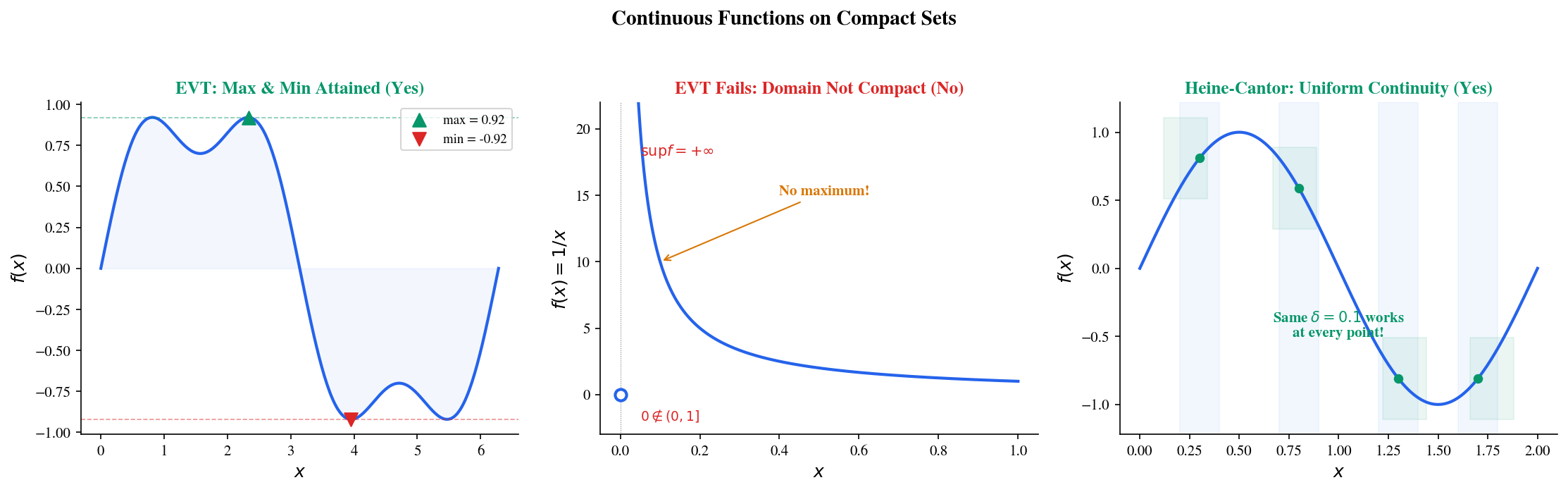
🔷 Theorem 4 (Extreme Value Theorem (Compactness Proof))
If is continuous and is compact, then attains its maximum and minimum on : there exist with for all .
Proof.
By Lemma 1, is compact, hence closed and bounded by Heine-Borel. Since is bounded, exists. Since is closed and is a limit point of (by the approximation property of the supremum: there exist with ), we have . So for some .
The argument for the minimum is identical with replacing .
Compare this with the proof in Epsilon-Delta & Continuity (Theorem 4): the compactness proof is cleaner because it identifies the essential structural ingredient. The continuous image of a compact set is compact — that is the entire story.
🔷 Theorem 5 (Heine-Cantor Theorem (Compactness Proof))
If is continuous and is compact, then is uniformly continuous on : for every , there exists such that for all .
Proof.
Suppose is not uniformly continuous. Then there exists such that for every , there exist with but .
By compactness of , the sequence has a subsequence . Since , we also have .
By continuity of at : so . But for all — contradiction.
💡 Remark 4
The Heine-Cantor proof by contradiction is a paradigm for compactness arguments: assume the negation, extract a sequence, use compactness to get a convergent subsequence, and reach a contradiction via continuity. This pattern — sometimes called the “compactness argument” — appears throughout analysis and optimization theory. Whenever you see a proof that constructs a sequence and extracts a convergent subsequence, compactness is at work.
Coercivity — Compactness Without Boundedness
In practice, parameter spaces are — not compact (unbounded). So the EVT does not apply directly: might not be attained. This is not an abstract concern — the function on has infimum 0 but never reaches it.
Coercivity provides an elegant substitute: if the function “blows up” at infinity, the optimization effectively takes place on a compact sublevel set.
📐 Definition 8 (Coercive Function)
A function is coercive if . Equivalently, for every , the sublevel set is bounded.
🔷 Theorem 6 (Weierstrass Theorem for Coercive Functions)
If is continuous and coercive, then attains its minimum: there exists with .
Proof.
Let . Choose a minimizing sequence with .
Since , we have for all sufficiently large . The sublevel set is:
- Bounded, by coercivity of .
- Closed, by continuity of (preimage of the closed set ).
So is compact by the Heine-Borel theorem, and the tail of lies in . By compactness, extract a subsequence . By continuity, .
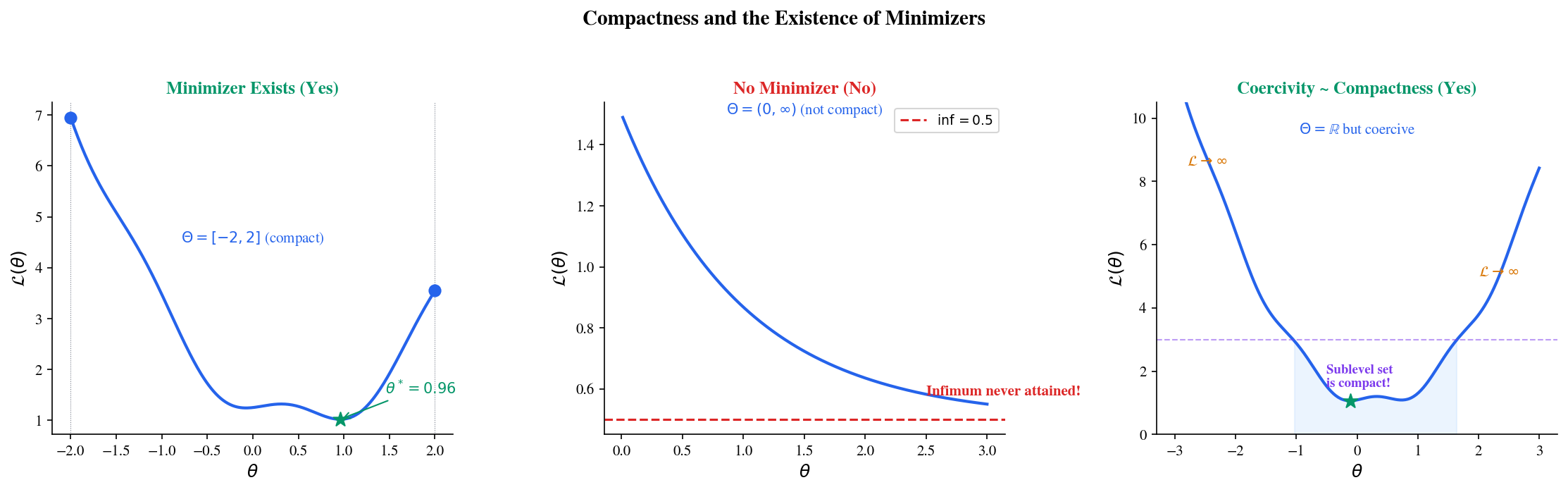
💡 Remark 5
Coercivity is why regularization guarantees a unique minimizer for convex losses. The regularized loss is coercive for any : the quadratic penalty dominates as , regardless of what does. The sublevel sets are compact (closed and bounded), so the Weierstrass theorem guarantees a minimizer exists. Without regularization, the loss might decrease asymptotically — approaching its infimum along a sequence with — without ever being attained.
Connections to Machine Learning
Regularization as compactification
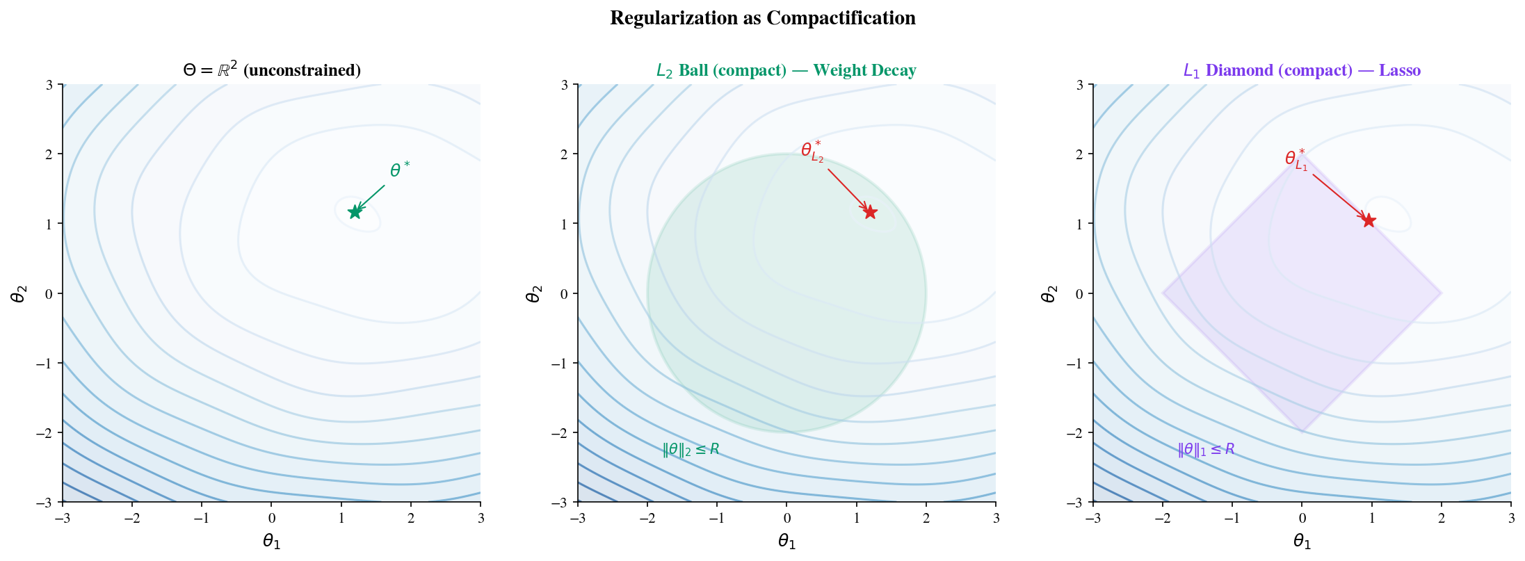
The unconstrained parameter space is not compact. Regularization techniques create compact subsets, restoring the EVT guarantee that minimizers exist:
- weight decay constrains , a closed ball in — compact by Heine-Borel.
- lasso constrains , a closed “diamond” (cross-polytope) — also compact.
- Elastic net combines both: — the intersection of compact sets, still compact.
- Weight clipping ( for all ) constrains parameters to a closed hypercube — compact.
- Spectral normalization constrains the spectral norm (largest singular value) of weight matrices, creating a compact set of matrices.
Each technique converts an unbounded optimization problem into a compact one, where the existence of minimizers is guaranteed by the EVT. Regularization is not just for generalization — it is for existence. See Convex Analysis on formalML for the full treatment.
Existence of optimal parameters
Without compactness or coercivity, may not be attained. Consider a simple example: on . The infimum is 0, but for all — the infimum is never achieved.
Regularization fixes this: is coercive for any , so its minimum is attained. The regularization parameter controls the trade-off between fitting the data and keeping parameters bounded — but at a more fundamental level, ensures the optimization problem has a solution. See Gradient Descent on formalML.
Tightness and convergence of distributions
Compactness appears in probability theory through the concept of tightness. A family of probability distributions is tight if for every , there exists a compact set such that for all . Prokhorov’s theorem says tightness is equivalent to sequential compactness of the family of measures (in the topology of weak convergence).
In ML, tightness guarantees that sequences of empirical distributions (from training data) have convergent subsequences — a key ingredient in proving that training procedures converge to meaningful distributions. See Measure-Theoretic Probability on formalML.
Early stopping and implicit compactness
Early stopping — halting training after iterations — implicitly constrains the effective parameter space. Starting from and taking gradient steps of size , the parameter trajectory is bounded: where is the maximum gradient norm. So the effective parameter space is contained in a ball of radius centered at — a compact set.
This observation connects early stopping to explicit regularization: both create compact constraint sets, and both guarantee that the optimization trajectory stays in a region where the EVT applies. The theoretical equivalence between early stopping and regularization (for linear models) is a manifestation of this shared compactness structure.
Computational Notes
Verifying the Nested Interval Property via bisection
import numpy as np

def nested_interval_bisection(a, b, target, max_steps=50):
    """Bisect [a, b] to locate target, returning interval history."""
    intervals = [(a, b)]
    for _ in range(max_steps):
        mid = (a + b) / 2
        if mid < target:
            a = mid
        else:
            b = mid
        intervals.append((a, b))
        if b - a < 1e-15:
            break
    return intervals

# Find √2 in [1, 2]
intervals = nested_interval_bisection(1, 2, np.sqrt(2), max_steps=50)
print(f"After {len(intervals)-1} steps: [{intervals[-1][0]:.15f}, {intervals[-1][1]:.15f}]")
print(f"Width: {intervals[-1][1] - intervals[-1][0]:.2e}")
print(f"√2 =   {np.sqrt(2):.15f}")
Demonstrating sequential compactness
def extract_convergent_subsequence(sequence, set_contains):
    """Extract a convergent subsequence and check if limit is in the set."""
    # Sort by value, take elements converging to the median
    sorted_vals = sorted(enumerate(sequence), key=lambda x: x[1])
    median_idx = len(sorted_vals) // 2
    target = sorted_vals[median_idx][1]

    # Greedily select elements approaching the target
    subseq_indices = [sorted_vals[median_idx][0]]
    for i in range(median_idx + 1, len(sorted_vals)):
        subseq_indices.append(sorted_vals[i][0])
    subseq_indices.sort()  # Restore original order

    subseq = [sequence[i] for i in subseq_indices[:20]]
    limit = np.mean(subseq[-5:])
    return subseq, limit, set_contains(limit)

# On [0, 1] (compact): limit stays in set
rng = np.random.default_rng(42)
seq = rng.uniform(0, 1, size=100)
subseq, limit, in_set = extract_convergent_subsequence(seq, lambda x: 0 <= x <= 1)
print(f"[0,1]: limit = {limit:.6f}, in set: {in_set}")

# On (0, 1) (not compact): limit might escape
seq = np.array([1/(n+1) for n in range(100)])  # converges to 0 ∉ (0,1)
subseq, limit, in_set = extract_convergent_subsequence(seq, lambda x: 0 < x < 1)
print(f"(0,1): limit = {limit:.6f}, in set: {in_set}")
Checking coercivity of regularized objectives
def check_coercivity(f, x_range, n_points=1000):
    """Check if f appears coercive by examining boundary behavior."""
    x = np.linspace(*x_range, n_points)
    y = np.array([f(xi) for xi in x])

    boundary = n_points // 10
    left_min = y[:boundary].min()
    right_min = y[-boundary:].min()
    interior_min = y[boundary:-boundary].min()

    is_coercive = left_min > interior_min and right_min > interior_min
    return is_coercive, y.min(), x[y.argmin()]

# Unregularized: L(θ) = e^(-θ²) — NOT coercive
coercive, fmin, xmin = check_coercivity(lambda x: np.exp(-x**2), (-10, 10))
print(f"exp(-x²): coercive = {coercive}, min ≈ {fmin:.6f} at x ≈ {xmin:.4f}")

# Regularized: L(θ) + λ‖θ‖² = e^(-θ²) + 0.1θ² — coercive
coercive, fmin, xmin = check_coercivity(lambda x: np.exp(-x**2) + 0.1*x**2, (-10, 10))
print(f"exp(-x²) + 0.1x²: coercive = {coercive}, min ≈ {fmin:.6f} at x ≈ {xmin:.4f}")
Connections & Further Reading
Prerequisites — topics you need first
Sequences, Limits & Convergence
Completeness was introduced informally via Cauchy sequences and the Bolzano-Weierstrass Theorem. This topic elevates those results from 'useful theorems' to 'structural consequences of a single axiom' — the least upper bound property.
Epsilon-Delta & Continuity
The Extreme Value Theorem and Heine-Cantor Theorem were proved in Topic 2 using ad-hoc arguments. Here we reprove them as immediate consequences of compactness, revealing the deeper structural reason they hold.
Where this leads — next in formalCalculus
On to formalStatistics — where this calculus powers inference
Empirical Processes
Prokhorov's theorem (tightness ⇔ precompactness in distribution) is the probabilistic lift of Heine–Borel / Bolzano–Weierstrass. Donsker's theorem is proven via finite-dimensional CLT plus tightness; tightness is the compactness half of the argument.
Kernel Density Estimation
Uniform consistency proofs for KDEs (sup_x |f̂_n(x) - f(x)| → 0) use Arzelà–Ascoli-style equicontinuity and compactness arguments on the class of kernel-convolved densities.
On to formalML — where this calculus powers ML
Convex Analysis
The Weierstrass extreme value theorem — continuous functions on compact sets attain their extrema — is the foundational existence result for convex optimization. Compactness of sublevel sets for coercive convex functions guarantees minimizers exist even on unbounded domains.
Measure Theoretic Probability
Tightness of probability measures (Prokhorov's theorem) is a compactness condition: a family of measures is tight if for every ε > 0, there exists a compact set K with μ(K) > 1 - ε for all μ in the family. This is used in convergence-in-distribution proofs.
Gradient Descent
The existence of minimizers for regularized objectives (L(θ) + λ‖θ‖²) follows from compactness arguments: the regularization term makes the effective objective coercive, so sublevel sets are compact, and the EVT guarantees a minimizer exists.
References
- book Abbott (2015). Understanding Analysis Chapters 2–3 on completeness and Chapter 3 on compact sets — the primary reference for the completeness-first approach to real analysis
- book Rudin (1976). Principles of Mathematical Analysis Chapter 2 on basic topology and Chapter 4 on compactness — the definitive treatment of Heine-Borel and its consequences
- book Tao (2016). Analysis I Chapter 12 on metric spaces and compactness — careful first-principles construction connecting completeness, compactness, and continuity
- book Boyd & Vandenberghe (2004). Convex Optimization Section 4.2 on existence of optimal solutions and Section 6.1 on regularization — direct applications of compactness to optimization
- book Folland (1999). Real Analysis Chapter 4 on topological spaces and Tychonoff's theorem — for readers wanting the general topological perspective
- paper Zou & Hastie (2005). “Regularization and Variable Selection via the Elastic Net” The elastic net combines L1 and L2 penalties — both create compact constraint sets, guaranteeing minimizer existence while promoting sparsity