Multiple Integrals & Fubini's Theorem
Extending integration to functions of several variables — double and triple integrals defined via multidimensional Riemann sums, Fubini's theorem reducing them to iterated single integrals, integration over general regions, and Monte Carlo methods for high-dimensional computation
Abstract. The Riemann integral integrates a function of one variable over an interval. Multiple integrals extend this to functions of several variables over regions in higher dimensions. The double integral over a rectangle R = [a,b] × [c,d] is defined via two-dimensional Riemann sums: partition R into sub-rectangles, evaluate f at sample points, sum the volume contributions, and take the limit as the mesh goes to zero. Fubini's Theorem is the computational engine: for continuous f, the double integral equals the iterated integral in either order. For non-rectangular regions, Fubini extends to Type I domains (vertical slices with variable y-limits) and Type II domains (horizontal slices with variable x-limits). Triple integrals extend the construction to three dimensions. In machine learning, multiple integrals are pervasive: joint densities, marginal densities obtained by integrating out variables, expected values, and covariance are all multiple integrals. When closed-form evaluation is impossible in high dimensions, Monte Carlo integration approximates by random sampling, connecting to the mini-batch strategy of SGD.
Overview & Motivation
In machine learning, the expected loss over a joint distribution of data and parameters is
This is a double integral — the function is integrated over two variables simultaneously. But how do we define this integral rigorously? And more importantly, how do we compute it?
The answer comes in two parts. First, we define the double integral as a limit of two-dimensional Riemann sums, directly generalizing the 1D construction from The Riemann Integral. Second, Fubini’s theorem tells us we can evaluate the double integral as two nested single integrals — and the order doesn’t matter (for continuous functions). This transforms a genuinely two-dimensional problem into a sequence of one-dimensional problems we already know how to solve.
This topic opens the Multivariable Integral Calculus track. We combine the integration machinery from The Riemann Integral & FTC with the partial-derivative perspective from Partial Derivatives & the Gradient: an iterated integral is “integrate with respect to , treating as constant” — precisely the partial-derivative viewpoint applied to integration rather than differentiation.
Double Integrals over Rectangles
We start where The Riemann Integral started — with Riemann sums — but now in two dimensions. The surface hovers above a rectangle in the -plane. We want to compute the “volume” between the surface and .
📐 Definition 1 (Partition of a Rectangle)
Let be a closed rectangle in . A partition of is a pair where
is a partition of and
is a partition of . This creates sub-rectangles , each with area .
The mesh (or norm) of the partition is — the larger of the two 1D meshes.
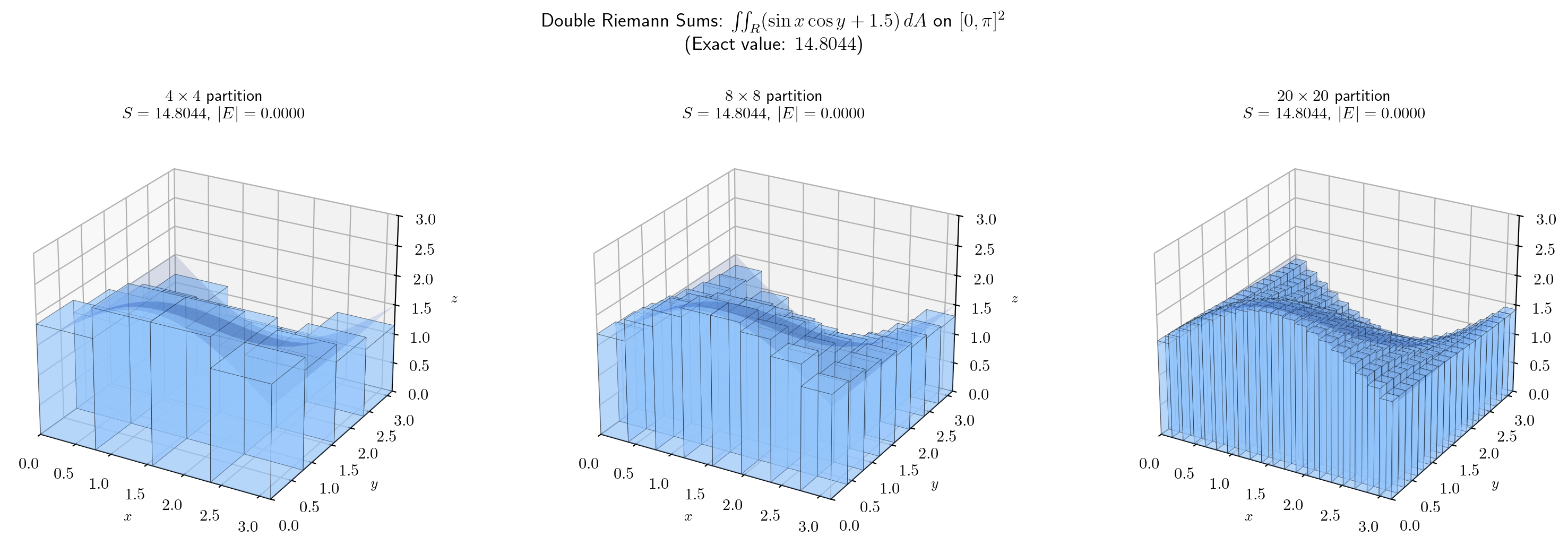
📐 Definition 2 (Double Riemann Sum)
Given a function , a partition of , and sample points in each sub-rectangle, the double Riemann sum is
Each term is the signed volume of a box with base and height .
📐 Definition 3 (The Double Integral)
The double integral of over is the limit of double Riemann sums as the mesh of the partition tends to zero:
provided this limit exists and is the same for all choices of sample points. When this limit exists, we say is integrable on .
💡 Remark 1 (Notation)
The notations , , and are all equivalent. The "" notation emphasizes the area element ; the "" notation makes the variables explicit. We use whichever is clearest in context.
📝 Example 1 (Constant Function: Area Computation)
Let on . Every Riemann sum equals
So , which is the area of . This generalizes the 1D fact that .
📝 Example 2 (f(x,y) = x + y on the Unit Square)
Let on . Using a uniform partition with subdivisions per axis and center sample points, the Riemann sum is
As , this converges to .
Try the interactive explorer below — increase and watch the boxes fill the volume:
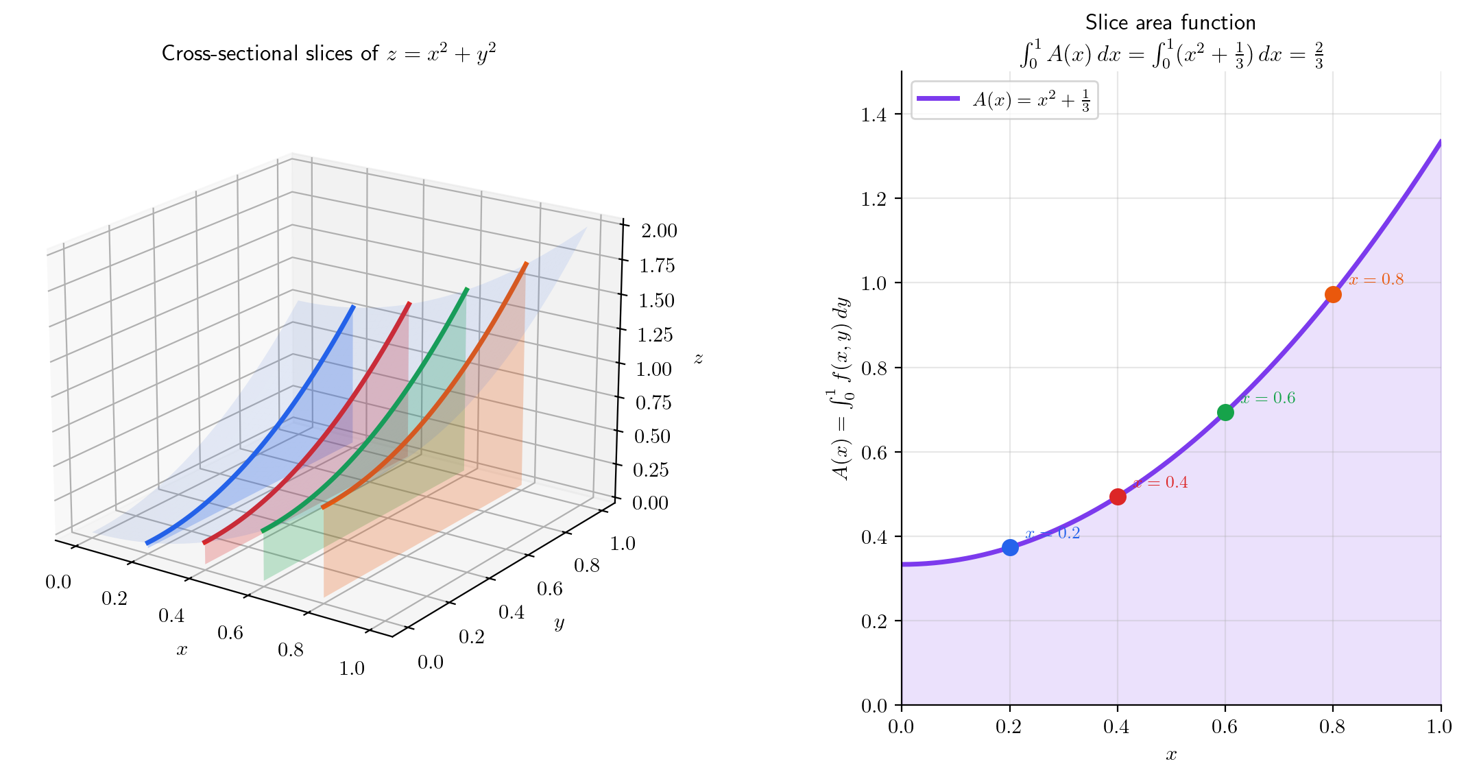
Iterated Integrals
Instead of computing a two-dimensional limit, can we reduce the double integral to a sequence of ordinary integrals? The idea is to integrate “one variable at a time.”
📐 Definition 4 (Iterated Integral)
Given , the iterated integral (with outer, inner) is
First, fix and integrate over to obtain the slice function . Then integrate over .
The iterated integral with the reversed order is .
📝 Example 3 (Iterated Integral of x + y)
Compute . Inner integral first:
Then the outer integral:
📝 Example 4 (Reversed Order Gives the Same Answer)
Now compute . Inner integral:
Outer integral:
Both orders give 1 — this is not a coincidence.
💡 Remark 2 (Cavalieri's Principle)
The slice function represents the cross-sectional area at position . The iterated integral sums these cross-sectional areas — this is precisely Cavalieri’s principle: the volume of a solid is the integral of its cross-sectional areas. Cavalieri stated this in 1635 as a geometric principle; we now prove it as a consequence of Fubini’s theorem.
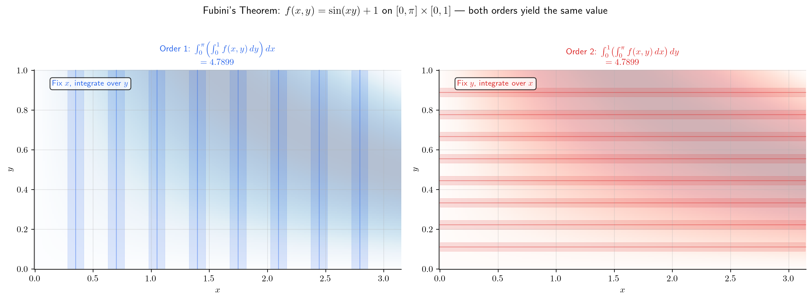
Fubini’s Theorem
This is the central result of this topic. It says that the double integral equals either iterated integral — the “two-dimensional” computation reduces to a pair of “one-dimensional” computations.
🔷 Theorem 1 (Fubini's Theorem (Rectangle Case))
Let be continuous. Then is integrable on , and
That is, the double integral equals the iterated integral in either order.
Proof.
We prove that . The equality with the other iterated integral follows by symmetry (swap the roles of and ).
Step 1: Integrability. Since is continuous on the compact set , it is uniformly continuous (Heine-Cantor theorem, Completeness & Compactness). In particular, is bounded on . For any , uniform continuity provides such that whenever . For any partition with , on each sub-rectangle :
where and are the supremum and infimum of on . Therefore the gap between upper and lower Darboux sums is
Since was arbitrary, is integrable on .
Step 2: The slice function is well-defined. For each fixed , the function is continuous on (since is continuous on ). By the 1D integrability theorem (The Riemann Integral, Theorem 1), is integrable, so the slice function
is well-defined for every .
Step 3: is continuous. We show is continuous using uniform continuity of . For the from Step 1:
If , then , so for all . Therefore . Since is continuous on , it is integrable.
Step 4: Squeeze. Take a partition with . For each sub-rectangle :
Summing over : for all . Integrating over :
Summing over all :
But also lies between and . Since and is arbitrary:
💡 Remark 3 (Fubini Beyond Continuity)
Fubini’s theorem extends well beyond continuous functions. The Fubini-Tonelli theorem applies to Lebesgue-integrable functions: if (or if ), then the iterated integrals exist and are equal to the double integral. The continuity hypothesis above is a convenient sufficient condition, but not necessary. The full generalization lives in measure theory — a topic for the Measure & Integration track (coming soon).
📝 Example 5 (∫∫ x sin(xy) dA over [0, π] × [0, 1])
Compute where .
dy-first: Fix . Inner integral:
Outer integral:
The other order (-first) requires integration by parts twice — both orders give , but -first is dramatically simpler.
Integration over General Regions
So far we’ve integrated over rectangles. Real applications require integration over non-rectangular regions — disks, triangles, regions bounded by curves.
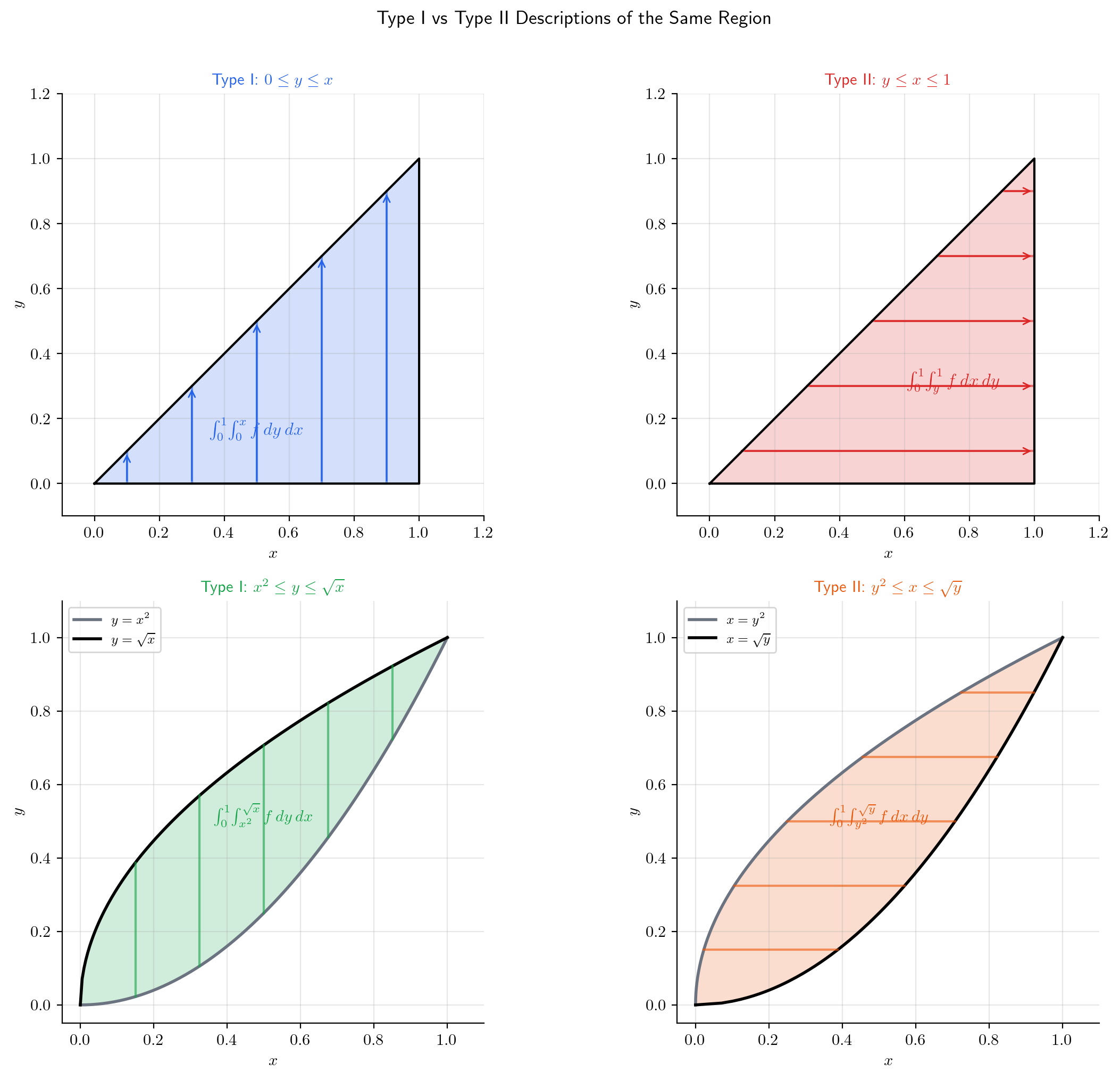
📐 Definition 5 (Type I Region)
A Type I region in is described by
where and are continuous on with . The -limits depend on — we slice with vertical strips.
📐 Definition 6 (Type II Region)
A Type II region is described by
where and are continuous on with . The -limits depend on — we slice with horizontal strips.
🔷 Theorem 2 (Fubini's Theorem (General Regions))
Let be continuous on a region .
If is Type I:
If is Type II:
If is both Type I and Type II, both iterated integrals are equal.
📝 Example 6 (Triangle: Both Orders)
Let — the triangle below the line .
Type I ( outer): ranges from to ; for each , ranges from to :
Type II ( outer): ranges from to ; for each , ranges from to :
Both give — the area of the triangle.
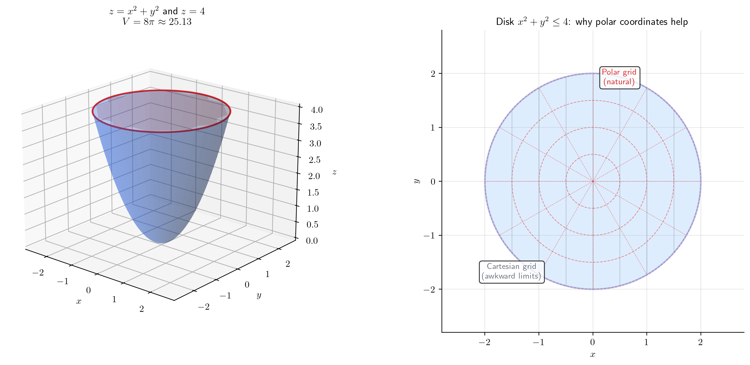
📝 Example 7 (Disk — Painful in Cartesian)
The area of the unit disk as a Type I integral:
This is computable (via substitution) but awkward. In polar coordinates the same integral becomes — trivially. This is the motivation for the next topic: Change of Variables & the Jacobian Determinant.
💡 Remark 4 (Regions That Are Neither Type I Nor Type II)
Some regions (e.g., an annulus, or an L-shaped domain) cannot be described as a single Type I or Type II region. The solution: decompose the region into finitely many pieces, each of which is Type I or Type II, and use the additivity property (Theorem 3 below). Alternatively, a change of coordinates (polar, cylindrical, spherical) may reduce the region to a simple rectangle in the new coordinates.
Choosing Integration Order
Sometimes one integration order leads to an impossible inner integral, while the other order is elementary. Recognizing this — and knowing how to reverse the order — is an essential computational skill.
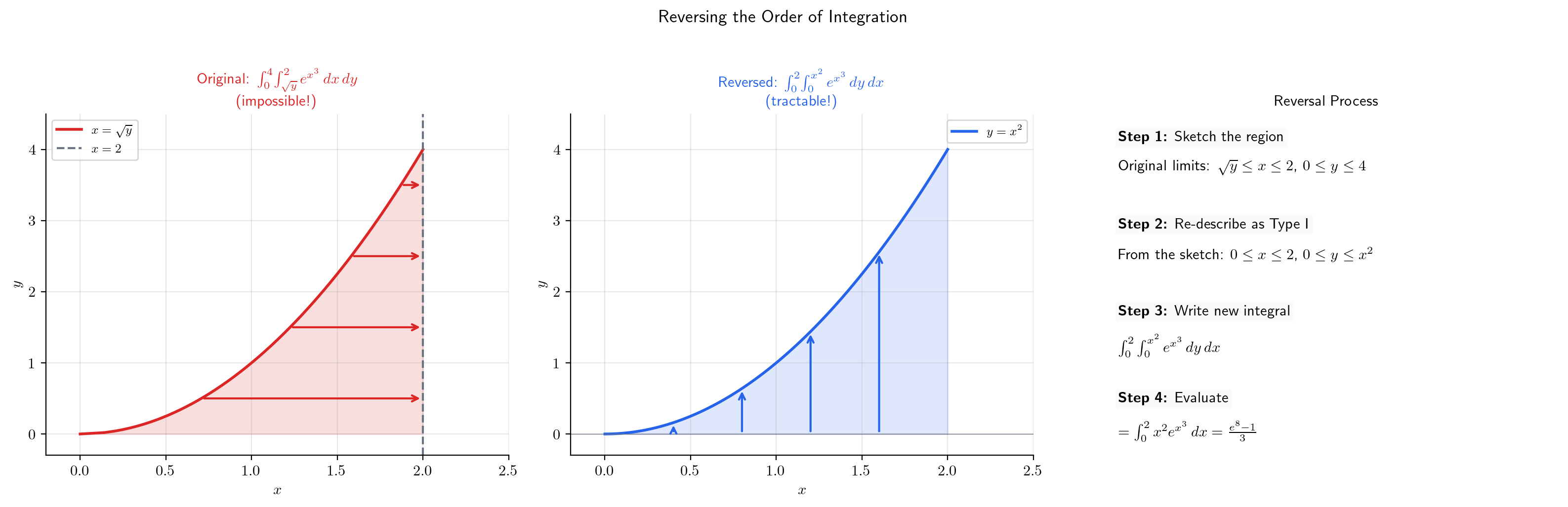
📝 Example 8 (e^{x³}: Impossible in One Order, Elementary in the Other)
Compute .
The inner integral has no closed-form antiderivative — cannot be integrated in terms of elementary functions. We are stuck.
Reverse the order. Sketch the region: , . Equivalently: , . In the reversed order:
The key move: the inner integral , and now is a perfect -substitution candidate with .
💡 Remark 5 (When to Switch Order)
Consider switching the integration order when:
- The inner integral has no elementary antiderivative.
- The limits in the current order are complicated but would simplify if swapped.
- The integrand factors nicely in the other variable.
The procedure: (1) sketch the region, (2) re-describe it as the other type (Type I ↔ Type II), (3) write the new limits, (4) evaluate.
Properties of Double Integrals
The double integral inherits the familiar properties of the 1D integral — linearity, monotonicity, additivity — because Fubini reduces it to 1D integrals.
🔷 Theorem 3 (Properties of the Double Integral)
Let be continuous on a region , and let . Then:
- Linearity:
- Monotonicity: If on , then
- Additivity: If with having zero area, then
- Triangle Inequality:
- Area:
Proof.
Each property follows from Fubini’s theorem + the corresponding 1D property. For example, linearity: by Fubini,
By linearity of the 1D integral (The Riemann Integral, Theorem 3), the inner integral splits:
Linearity of the outer integral then gives
The other properties follow similarly — monotonicity from the 1D monotonicity property, additivity from additivity of 1D integrals over adjacent intervals, and the triangle inequality from and monotonicity.
🔷 Proposition 1 (Mean Value Theorem for Double Integrals)
If is continuous on a connected, bounded region with , then there exists a point such that
In other words, attains its average value somewhere in .
Proof.
Since is continuous on the compact set , the Extreme Value Theorem (Completeness & Compactness) gives for all , where and are the minimum and maximum of on . By monotonicity of the integral:
Dividing by :
The quantity in the middle lies between and for some . Since is connected and is continuous, the Intermediate Value Theorem guarantees there exists with .
Triple Integrals and Higher Dimensions
The construction extends naturally to three (and more) dimensions. We partition a box into sub-boxes, form Riemann sums with volume elements , and take the limit.
📐 Definition 7 (Triple Integral)
The triple integral of over a region is
Fubini’s theorem extends: for continuous , the triple integral equals any of the six possible iterated integrals (three nested single integrals in any order of the three variables).
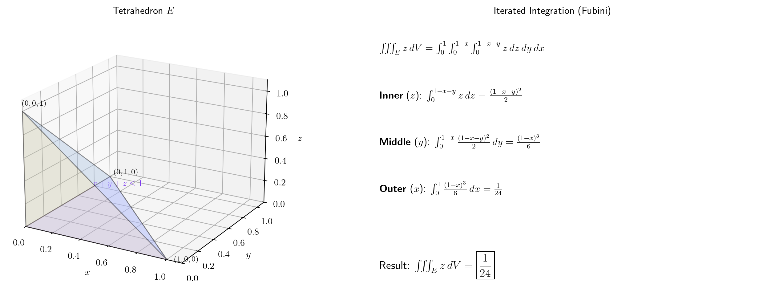
📝 Example 9 (Volume of a Tetrahedron)
Compute where — the standard tetrahedron.
Set up as a Type-I-style iterated integral: ranges from to ; for each , ranges from to ; for each , ranges from to .
Innermost:
Middle: Substituting :
Outer:
💡 Remark 6 (The Curse of Dimensionality)
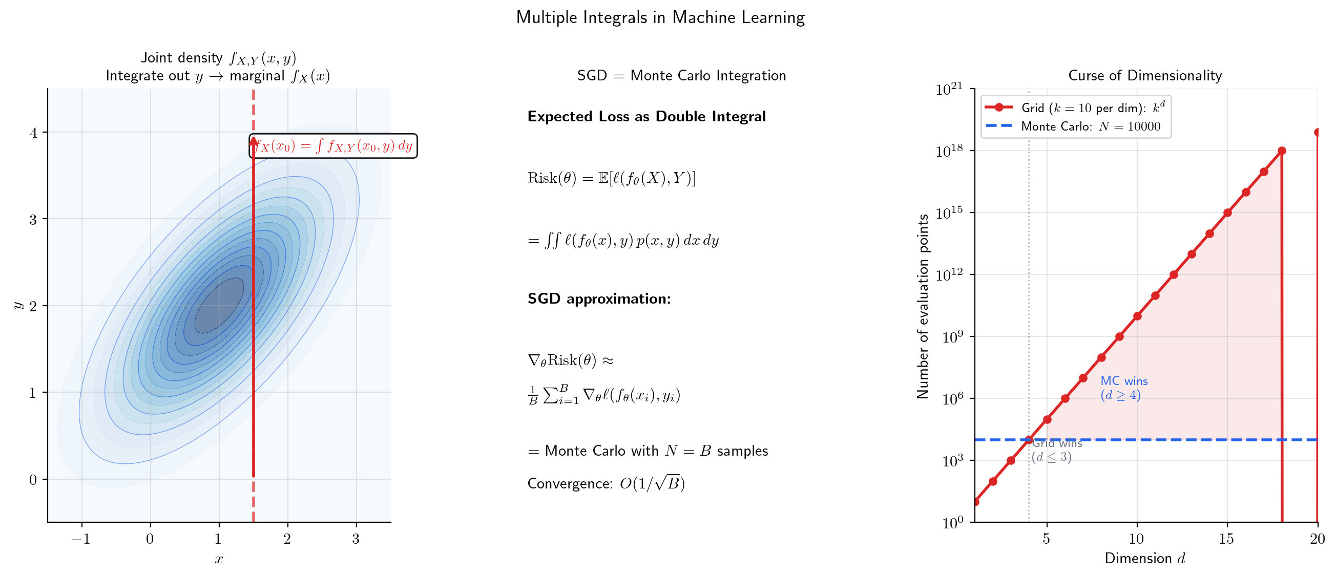
For a product-rule grid in dimensions with points per axis, the total number of evaluations is . With and , that’s evaluations — far beyond any computer. This exponential scaling is the curse of dimensionality. It’s why the ML integrals over 10,000-dimensional parameter spaces don’t use quadrature. They use Monte Carlo — next section.
Monte Carlo Integration
When deterministic quadrature fails (high dimensions, complex regions), we turn to randomness. Monte Carlo integration replaces systematic grids with random samples.
📐 Definition 8 (Monte Carlo Estimate)
Let be a region with volume , and let be independent, uniformly distributed random points in . The Monte Carlo estimate of is
This is the sample mean of scaled by the volume of .
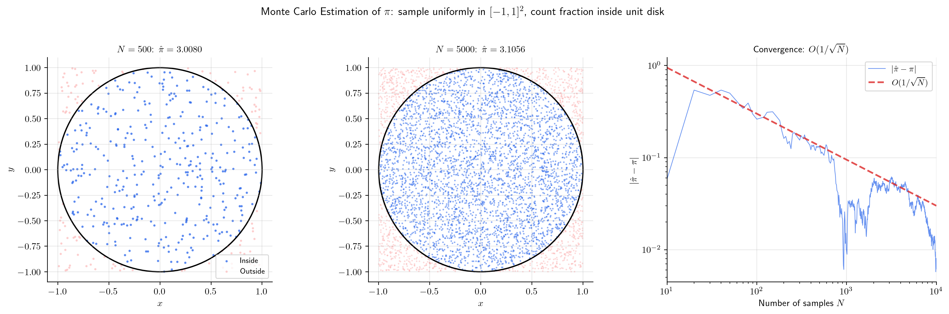
🔷 Proposition 2 (Monte Carlo Error)
The Monte Carlo estimate is unbiased: . Its standard error is
where is the variance of over . The convergence rate is — independent of dimension. This is why Monte Carlo wins in high dimensions.
Proof.
Sketch. Since the are i.i.d. uniform on , . So
The variance: .
Taking square root gives the standard error .
📝 Example 10 (Estimating π via Monte Carlo)
The area of the unit disk is . Inscribe it in the square (area 4). Sample uniform points in the square. The fraction inside the disk estimates :
With points, we typically get . Try it below:
💡 Remark 7 (Monte Carlo vs. Quadrature — and SGD)
In dimensions, quadrature needs evaluations for accuracy (for the trapezoidal rule). Monte Carlo needs evaluations for accuracy — and is independent of . For or so, Monte Carlo dominates.
This is exactly why stochastic gradient descent (SGD) uses random mini-batches. The expected risk is a high-dimensional integral. Each mini-batch of size is a Monte Carlo estimate with error .
→ Gradient Descent on formalML
Connections to Statistics
Joint densities, marginal distributions, posterior normalizing constants, MISE — every multivariable probabilistic computation is a multiple integral. Fubini and the change-of-variables theorem do the work behind the scenes.
Joint and marginal densities
A joint density integrates to over — a multivariate integral. Marginalizing is an iterated integral (justified by Fubini). The multivariate Normal normalizer comes from the multivariate Gaussian integral. See formalStatistics Multivariate Distributions.
Bayesian normalizing constants and MCMC
The posterior has a normalizing integral over the parameter space. In dimensions this is a -dimensional integral; MCMC is the strategy for approximating it when is too large for deterministic quadrature. See formalStatistics Bayesian Foundations & Prior Selection and formalStatistics Bayesian Computation & MCMC.
Hierarchical models and KDE
Hierarchical-model marginal likelihoods integrate over the individual-level parameter. The KDE MISE is a multi-dimensional integral whose bias-variance decomposition uses Fubini to swap expectation and spatial integration. See formalStatistics Hierarchical Bayes & Partial Pooling and formalStatistics Kernel Density Estimation.
Connections to ML
Multiple integrals are not just mathematical machinery — they are the language of probability and statistical learning.
Joint and Marginal Densities
A joint density satisfies . The marginal density of is obtained by “integrating out” :
This is Fubini applied to probability. Every time you marginalize — whether computing the marginal likelihood in Bayesian inference or the evidence lower bound (ELBO) in variational inference — you’re invoking Fubini’s theorem.
→ Measure-Theoretic Probability on formalML
Expected Values and Covariance
The expected value of a function under a joint density is
Covariance is: — each term a double integral, simplified by Fubini + linearity.
Monte Carlo Estimation and SGD
The expected risk is a double integral we can’t compute (we don’t know ). Each SGD mini-batch of size is a Monte Carlo estimate:
with standard error . Larger batches reduce variance but cost more computation — the fundamental trade-off of stochastic optimization.
→ Gradient Descent on formalML
Partition Function in Energy-Based Models
In models like the Boltzmann machine, the partition function is an intractable integral over a high-dimensional space. Contrastive divergence and other training methods are essentially schemes for estimating ratios of such integrals without computing them directly.
Preview: Change of Variables
The Gaussian integral is proved by converting to polar coordinates — a change of variables that transforms the double integral into a simpler form. The general theory requires the Jacobian determinant as a volume scaling factor. The full proof appears in Change of Variables & the Jacobian Determinant, §5.
Connections & Further Reading
Prerequisites — topics you need first
The Riemann Integral & FTC
The double integral generalizes the 1D Riemann sum construction. Fubini reduces double integrals to nested single integrals. All proofs rely on 1D integral properties.
Partial Derivatives & the Gradient
Iterated integration uses the partial-derivative perspective: integrate with respect to y while treating x as constant.
Epsilon-Delta & Continuity
Uniform continuity on compact rectangular domains (Heine-Cantor) is the key hypothesis in Fubini's proof.
Completeness & Compactness
Compactness of R = [a,b] × [c,d] ensures continuous functions are bounded and uniformly continuous.
Improper Integrals & Special Functions
The Gaussian integral proof via polar coordinates is revisited as a motivating example for change of variables.
The Jacobian & Multivariate Chain Rule
The Jacobian determinant appears in the next topic (Change of Variables) as the volume scaling factor.
Where this leads — next in formalCalculus
On to formalStatistics — where this calculus powers inference
Multivariate Distributions
A joint density f(x_1,...,x_n) integrates to 1 over ℝⁿ — a multivariate integral. Marginalizing f_i(x_i) = ∫ f(x_1,...,x_n) dx_{-i} is an iterated integral (justified by Fubini). The multivariate Normal normalizer (2π)^(d/2) √det Σ comes from the multivariate Gaussian integral.
Bayesian Foundations And Prior Selection
The posterior p(θ|x) = p(x|θ)π(θ) / ∫ p(x|θ)π(θ) dθ has a normalizing integral over the full parameter space. In d dimensions this is a d-dimensional integral; Fubini justifies iterated computation when possible.
Bayesian Computation And MCMC
MCMC is a strategy for approximating d-dimensional integrals when d is too large for deterministic quadrature. The target is always an expectation ∫ g(θ) p(θ|x) dθ, and the sampler converts this into an ergodic-average approximation.
Hierarchical Bayes And Partial Pooling
The hierarchical-model marginal likelihood p(x|φ) = ∫ p(x|θ) p(θ|φ) dθ integrates over the individual-level parameter θ. Full Bayes integrates further over φ. These nested integrals define the partial-pooling structure.
Kernel Density Estimation
The MISE E[∫ (f̂_n(x) - f(x))² dx] is a multi-dimensional integral over the support. The bias-variance decomposition uses Fubini to swap expectation and spatial integration.
Order Statistics And Quantiles
Joint densities of order statistics are multi-dimensional integrals; computing E[X_{(k)}] requires integrating over the (n-1)-simplex of order constraints. Marginal densities of individual order statistics fall out of these multivariate integrals via Fubini.
Bayesian Model Comparison And Bma
Topic 27's Laplace expansion of the marginal likelihood $m(\mathbf{y}) = \int L(\theta)\pi(\theta)\,d\theta$ uses multivariate Gaussian integration over a neighborhood of the posterior mode (a $d$-dimensional integral); §27.6 Proof 2 invokes the iterated-integral/determinant machinery developed here.
On to formalML — where this calculus powers ML
Measure Theoretic Probability
Joint densities and marginals are computed via Fubini's theorem. Every two-variable probabilistic computation is a multiple integral. The Fubini-Tonelli theorem generalizes this to Lebesgue integrals.
Bayesian Nonparametrics
Multi-parameter posteriors require integrating over high-dimensional parameter spaces. Fubini enables Gibbs sampling, and Monte Carlo methods estimate intractable integrals.
Gradient Descent
The expected risk is a double integral over the joint distribution. Each SGD mini-batch is a Monte Carlo estimate. Monte Carlo error bounds inform stochastic gradient variance.
Causal Inference Methods
The §3.4 g-formula functional $\mathbb{E}_X[\mu_1(X) - \mu_0(X)] = \int (\mu_1(x) - \mu_0(x))\,dF_X(x)$ is an explicit multivariate integral over the covariate distribution. The longitudinal extension in §14.2 iterates this integral across time-points, requiring the Fubini machinery developed in this topic.
High Dimensional Regression
Sub-Gaussian tail bounds and union-bound deviation inequalities in the §5.5 lasso oracle inequality use multivariable-integration moves to control $\|\mathbf{X}^\top \boldsymbol\varepsilon / n\|_\infty$. The high-dimensional concentration substrate sits on the multiple-integral framework.
Kernel Regression
The bias-variance asymptotics in §§3–4 integrate the kernel against the design density $f_X(x)\,dx$ on the support of $X$. The change-of-variables substitution $u = (z - x)/h$ in §3.2 and the $d$-dimensional volume scaling $h^d$ in §6.3 are standard multivariate-integration moves; §6.1's product kernel $R(K) = R(K_1)^d$ uses Fubini.
Local Regression
Multivariate-integration substrate for the §4 bias-variance computations and the §8 multivariate full-degree expansion. The change-of-variables $u = (z - x)/h$ that converts kernel-weighted moments into kernel-moment integrals, and the boundary-truncated form $\mu_j^{(c)} = \int_{-c}^{\infty}$, are standard multivariate-integration moves used throughout the bias derivations.
Sparse Bayesian Priors
Sparse Bayesian priors' §2 scale-mixture-of-Normals representation marginalizes local scales $\lambda_j$ out of the joint prior — a multivariate Lebesgue integral over the $(\lambda_1, \ldots, \lambda_p, \tau)$ hyperparameter space. The Polson–Scott sparsity characterization (Theorem 1) of $p(\beta_j)$ presupposes the iterated-integral identity developed here.
Statistical Depth
Statistical depth's halfspace mass $F(H)$ and functional-band mass $F(B)$ are concrete multivariate integrals over closed halfspaces and bands; the §§2–5 derivations and Proposition 1's convexity proof use Fubini-style iterated integration over those regions.
References
- book Spivak (1965). Calculus on Manifolds Chapter 3 — Riemann integral in Rⁿ via partitions and Fubini's theorem
- book Rudin (1976). Principles of Mathematical Analysis Chapter 10 — rigorous treatment of multiple integrals via iterated integration
- book Munkres (1991). Analysis on Manifolds Chapters 2-3 — Riemann integration in Rⁿ with measurability conditions for Fubini
- book Hubbard & Hubbard (2015). Vector Calculus, Linear Algebra, and Differential Forms Chapter 4 — geometric motivation and computational techniques for multiple integrals
- book Bishop (2006). Pattern Recognition and Machine Learning Chapter 2 — marginal, conditional, and joint densities via multiple integrals