Measure & Integration · advanced · 50 min read

The Lebesgue Integral

Building the integral that handles limits — from simple function construction through the convergence theorems that make measure theory the engine of modern probability and machine learning.

Abstract. The Lebesgue integral is the completion of a promise. Topic 25 built the framework — sigma-algebras, measures, measurable functions, simple functions — but stopped short of the payoff: an integral powerful enough to handle limits. The Riemann integral fails when you need to interchange a limit and an integral, which is exactly what probability theory and machine learning do constantly. The Lebesgue integral fixes this. We construct it in three stages: first, for simple functions (finite sums weighted by measures); second, for non-negative measurable functions (supremum over simple approximations from below); and third, for general measurable functions (splitting into positive and negative parts). The three convergence theorems — Monotone Convergence, Fatou's Lemma, and Dominated Convergence — are the reason this integral exists. Dominated Convergence, in particular, is the mathematical justification for every 'swap the gradient and expectation' move in stochastic optimization. Fubini's theorem extends the integral to product spaces, making iterated integration rigorous. Expected value, KL divergence, and the ELBO are all Lebesgue integrals — this topic makes that precise.

Where this leads → formalML

formalML Expected value E[X] = ∫ X dP is a Lebesgue integral against a probability measure. Every moment, MGF, and characteristic function computation is an application of this topic.
formalML The interchange ∇E[L(θ,X)] = E[∇L(θ,X)] in SGD convergence proofs is a Dominated Convergence Theorem application — the single most important ML use of this topic.
formalML KL divergence D_KL(P||Q) = ∫ log(dP/dQ) dP and cross-entropy are Lebesgue integrals against probability measures. Their properties (non-negativity, convexity) follow from integral inequalities.
formalML The ELBO is an integral identity derived from Jensen's inequality applied to a Lebesgue integral: log p(x) ≥ ∫ q(z) log[p(x,z)/q(z)] dz.

1. Three Puzzles the Lebesgue Integral Solves

Topic 25 built the measure-theoretic framework — sigma-algebras, measures, measurable functions, simple functions, null sets, “almost everywhere” — but stopped short of the actual payoff: an integral. We had the vocabulary in place to talk about integration in a measure-theoretic way, but no integral defined yet. This topic builds it.

The motivation is the same one that drove the original development of the theory in the early twentieth century. The Riemann integral, beautiful as it is, fails on three different kinds of question that we routinely need to answer in probability theory and machine learning. Each failure points at a property we need the new integral to have.

If the proofs in this topic feel more technically demanding than Topic 25, that’s accurate — we are now working with suprema of integrals and interchanges of limits, which is where measure theory earns its keep. The conceptual mode is the same (sets, measures, measurable functions), but the manipulations are harder. Expect to slow down at the convergence-theorem proofs.

Puzzle 1: The limit–integral interchange failure

Define a sequence of functions $f_n: [0, 1] \to \mathbb{R}$ by $f_n(x) = n \cdot \mathbf{1}_{[0, 1/n]}(x).$

Each $f_n$ is a simple function: it equals $n$ on the interval $[0, 1/n]$ and $0$ elsewhere. The Riemann integral is well-defined for every $f_n$ and equals $\int_0^1 f_n(x) \, dx = n \cdot \frac{1}{n} = 1.$

So the integrals are constant: $\int_0^1 f_n = 1$ for every $n$ .

Now look at the pointwise limit. For any fixed $x \in (0, 1]$ , eventually $1/n < x$ — specifically, for $n > 1/x$ — and so $f_n(x) = 0$ for all sufficiently large $n$ . At $x = 0$ , $f_n(0) = n$ for every $n$ , so $f_n(0) \to \infty$ — a single point we can ignore. Putting these together, $\lim_{n \to \infty} f_n(x) = 0 \quad \text{for every } x \in (0, 1].$

So the pointwise limit $f$ equals $0$ almost everywhere, and any reasonable theory of integration should give $\int_0^1 f = 0$ .

But $\lim_{n \to \infty} \int_0^1 f_n = 1 \neq 0 = \int_0^1 \lim_{n \to \infty} f_n$ .

The Riemann integral provides no theorem that tells us when we are allowed to swap a limit and an integral. We are simply forbidden from doing it without justification, and there is no general justification available.

📝 Example 1 (The limit–integral interchange failure)

The sequence $f_n(x) = n \cdot \mathbf{1}_{[0, 1/n]}(x)$ on $[0, 1]$ has pointwise limit $f(x) = 0$ (for every $x > 0$ ), but $\int_0^1 f_n(x) \, dx = 1 \quad \text{for every } n, \qquad \int_0^1 f(x) \, dx = 0.$

This is the simplest possible witness that “limit of integrals” and “integral of limit” can disagree. The mass of $f_n$ — concentrated on a thin spike near $x = 0$ — does not vanish in the limit, even though the spike itself does.

The Lebesgue integral comes with a precise theorem — the Dominated Convergence Theorem — that tells us exactly when the swap is legal: if $|f_n| \leq g$ for some integrable function $g$ , the swap is valid. The sequence above escapes every dominating function (any $g$ would have to satisfy $g \geq n$ on $[0, 1/n]$ for every $n$ , forcing $g$ to be unbounded near $0$ in a non-integrable way), so its failure is not a defect of the theory but a genuine warning. By the end of Section 7 we’ll see this tightness from both sides: scenarios where DCT applies and the swap is valid, and the spike sequence above as a textbook example of what happens when the domination hypothesis fails.

Puzzle 2: The mixture distribution

Suppose a random variable $X$ has the following law: with probability $1/2$ it equals exactly $0$ (a point mass), and with probability $1/2$ it is drawn from the exponential density $p(x) = e^{x}$ on $(-\infty, 0)$ . Computing the expected value $E[X]$ requires integrating against a measure that is neither purely absolutely continuous nor purely discrete.

Try to write this expectation as a Riemann integral. The continuous part contributes $\frac{1}{2} \int_{-\infty}^0 x \cdot e^{x} \, dx,$ which is a perfectly fine improper Riemann integral and evaluates to $-1/2$ . But the point mass at $0$ contributes $0 \cdot \frac{1}{2} = 0$ to the expectation, and there is no way to capture that ” $0$ with probability $1/2$ ” inside a Riemann integral framework — the value of any Riemann integral over a single point is always zero, regardless of how much probability is concentrated there.

In the Lebesgue framework, the entire expectation is one integral against a single mixed measure $\mu = \frac{1}{2} \lambda|_{(-\infty, 0)} \cdot e^x + \frac{1}{2} \delta_0$ : $E[X] = \int x \, d\mu(x) = -\frac{1}{2} + 0 = -\frac{1}{2}.$

The point is not the numerical answer (which is the same either way — we got lucky here because $0$ contributes zero). The point is that the framework handles continuous and discrete components uniformly, with no special-case grafting. Mixtures of densities and atoms are everywhere in real-world ML — quantized neural networks, censored data, discrete-continuous outcome models — and the Lebesgue integral is what makes them legal mathematics rather than ad-hoc bookkeeping.

Puzzle 3: The gradient–expectation swap in SGD

When you train a model with stochastic gradient descent, the move at the heart of the algorithm is $\nabla_\theta \, E[L(\theta, X)] \;=\; E[\nabla_\theta L(\theta, X)].$

The left side is “differentiate the population loss”; the right side is “average the per-sample gradients.” We use this identity every time we compute a minibatch gradient and call it an unbiased estimator of the population gradient.

Look closely at what is being claimed. The gradient $\nabla_\theta$ is a limit (it’s the limit of difference quotients in $\theta$ ). The expectation $E[\,\cdot\,] = \int \cdot \, dP$ is an integral. So the identity is $\lim_{h \to 0} \int \frac{L(\theta + h, X) - L(\theta, X)}{h} \, dP(X) \;=\; \int \lim_{h \to 0} \frac{L(\theta + h, X) - L(\theta, X)}{h} \, dP(X).$

This is exactly a “limit of integrals equals integral of limit” claim. Without a convergence theorem, swapping the limit and the integral is just wishful thinking. The Dominated Convergence Theorem provides the conditions under which the swap is legal: if there exists an integrable $g(X)$ such that $|\nabla_\theta L(\theta, X)| \leq g(X)$ for all $\theta$ in a neighborhood, the interchange is valid.

In practice, ML papers cite this without naming it. Bounded gradients (gradient clipping), Lipschitz losses, and bounded-support data distributions are all ways to manufacture an integrable dominator. Every single SGD convergence proof in the literature implicitly invokes DCT at this step. Forward link: Gradient Descent.

Three failures, three needs: a convergence theorem for limits and integrals, a unified treatment of mixed measures, and a justification for swapping derivatives with expectations. The Lebesgue integral delivers on all three, and the rest of this topic shows how.

2. The Integral for Simple Functions

We start at the foundation. Recall from Topic 25 that a simple function on a measure space $(\Omega, \mathcal{F}, \mu)$ is a function of the form $s(x) = \sum_{k=1}^m c_k \cdot \mathbf{1}_{A_k}(x),$ where $c_1, \ldots, c_m$ are real numbers, $A_1, \ldots, A_m \in \mathcal{F}$ are measurable sets, and the $A_k$ partition (or at least cover) the relevant part of $\Omega$ . A simple function takes only finitely many distinct values, each on a measurable set.

We already know what simple functions are. Now we give them an integral. The definition is the only reasonable one: if $s$ takes value $c_k$ on the measurable set $A_k$ , then the integral of $s$ should be $\sum c_k \, \mu(A_k)$ — the “height times width” principle, with “width” measured by $\mu$ instead of by interval length.

📐 Definition 1 (Lebesgue integral of a non-negative simple function)

Let $(\Omega, \mathcal{F}, \mu)$ be a measure space and let $s = \sum_{k=1}^m c_k \cdot \mathbf{1}_{A_k}$ be a non-negative simple function ( $c_k \geq 0$ , $A_k \in \mathcal{F}$ , the $A_k$ disjoint). The Lebesgue integral of $s$ with respect to $\mu$ is $\int s \, d\mu \;=\; \sum_{k=1}^m c_k \cdot \mu(A_k),$ with the convention $0 \cdot \infty = 0$ (so a coefficient of zero on an infinite-measure set contributes zero, not “indeterminate”).

The convention $0 \cdot \infty = 0$ is essential. Without it, we couldn’t integrate the zero function over an infinite-measure space. With it, $\int 0 \, d\mu = 0$ for every measure $\mu$ , which is exactly what we want.

📝 Example 2 (The Dirichlet function has Lebesgue integral 0)

Take $\mu = \lambda$ (Lebesgue measure on $\mathbb{R}$ ) and $s = \mathbf{1}_{\mathbb{Q} \cap [0, 1]}$ . This is a simple function: it takes value $1$ on $\mathbb{Q} \cap [0, 1]$ and value $0$ on the rest of $[0, 1]$ . From Topic 25, every countable set has Lebesgue measure zero, so $\lambda(\mathbb{Q} \cap [0, 1]) = 0$ . The integral is $\int \mathbf{1}_{\mathbb{Q}} \, d\lambda \;=\; 1 \cdot \lambda(\mathbb{Q} \cap [0, 1]) + 0 \cdot \lambda([0, 1] \setminus \mathbb{Q}) \;=\; 1 \cdot 0 + 0 \cdot 1 \;=\; 0.$ This is the answer the Riemann integral could not give us. Topic 25’s opening puzzle is now closed: the Dirichlet function is Lebesgue-integrable, and its integral is exactly the value our intuition demanded.

📝 Example 3 (Integration against a Dirac measure evaluates at the point)

Let $\delta_a$ be the Dirac measure at $a \in \mathbb{R}$ : $\delta_a(A) = 1$ if $a \in A$ and $0$ otherwise. For any simple function $s = \sum c_k \mathbf{1}_{A_k}$ , $\int s \, d\delta_a \;=\; \sum_{k=1}^m c_k \cdot \delta_a(A_k) \;=\; c_{k(a)},$ where $k(a)$ is the unique $k$ with $a \in A_k$ . In other words, integrating against $\delta_a$ just evaluates the function at $a$ : $\int s \, d\delta_a = s(a)$ . This generalizes to all measurable functions in the next section, and it is the precise mathematical sense in which a “point mass” picks out a single value.

The integral of simple functions has exactly the algebraic structure we want — it is linear in the function and monotonic with respect to pointwise inequalities. The proof is a straightforward but careful unwinding of the definition.

🔷 Theorem 1 (Linearity and monotonicity for simple functions)

Let $s, t$ be non-negative simple functions on $(\Omega, \mathcal{F}, \mu)$ and $\alpha, \beta \geq 0$ . Then $\alpha s + \beta t$ is a non-negative simple function and $\int (\alpha s + \beta t) \, d\mu \;=\; \alpha \int s \, d\mu + \beta \int t \, d\mu.$ Moreover, if $s \leq t$ pointwise (or even just $\mu$ -a.e.), then $\int s \, d\mu \;\leq\; \int t \, d\mu.$

Proof.

We prove linearity first; monotonicity follows from it.

Step 1: A common refinement. Suppose $s = \sum_{i=1}^m a_i \mathbf{1}_{A_i}$ and $t = \sum_{j=1}^n b_j \mathbf{1}_{B_j}$ , where the $A_i$ partition the support of $s$ and the $B_j$ partition the support of $t$ . Form the joint refinement consisting of the sets $C_{ij} = A_i \cap B_j$ . These are measurable (intersections of measurable sets), pairwise disjoint, and they cover the union of supports. On each $C_{ij}$ , $s$ takes the constant value $a_i$ and $t$ takes the constant value $b_j$ , so $\alpha s + \beta t$ takes the constant value $\alpha a_i + \beta b_j$ . We have rewritten everything on a single common partition.

Step 2: Compute on the refinement. With everything on the refinement, the integrals are sums: $\int s \, d\mu \;=\; \sum_{i, j} a_i \cdot \mu(C_{ij}),$ $\int t \, d\mu \;=\; \sum_{i, j} b_j \cdot \mu(C_{ij}),$ $\int (\alpha s + \beta t) \, d\mu \;=\; \sum_{i, j} (\alpha a_i + \beta b_j) \cdot \mu(C_{ij}).$

The first and second sums recover the original definitions of $\int s \, d\mu$ and $\int t \, d\mu$ because $\sum_j \mu(C_{ij}) = \mu(A_i)$ by additivity of $\mu$ on the disjoint $\{C_{ij}\}_j$ , and similarly for $B_j$ . The third sum splits as $\sum_{i, j} (\alpha a_i + \beta b_j) \cdot \mu(C_{ij}) \;=\; \alpha \sum_{i, j} a_i \cdot \mu(C_{ij}) + \beta \sum_{i, j} b_j \cdot \mu(C_{ij}) \;=\; \alpha \int s \, d\mu + \beta \int t \, d\mu.$

That is linearity.

Step 3: Monotonicity. Suppose $s \leq t$ pointwise. On the common refinement, this means $a_i \leq b_j$ for every $C_{ij}$ with $\mu(C_{ij}) > 0$ . (If $\mu(C_{ij}) = 0$ the term contributes nothing.) Summing over $i, j$ : $\int s \, d\mu \;=\; \sum_{i, j} a_i \cdot \mu(C_{ij}) \;\leq\; \sum_{i, j} b_j \cdot \mu(C_{ij}) \;=\; \int t \, d\mu.$

If $s \leq t$ only $\mu$ -almost everywhere — that is, the set $\{x : s(x) > t(x)\}$ has measure zero — then on the common refinement the offending $C_{ij}$ values have $\mu(C_{ij}) = 0$ and contribute zero to both sums. The same chain of inequalities goes through.

∎

💡 Remark 1 (Well-definedness of the simple-function integral)

The definition $\int s \, d\mu = \sum c_k \mu(A_k)$ depends on the representation $s = \sum c_k \mathbf{1}_{A_k}$ that we chose. A given simple function has many such representations — we could refine the $A_k$ further, or we could merge sets that share the same coefficient. The proof above shows that the value $\int s \, d\mu$ is independent of representation: any two representations have a common refinement, and the integral computed on the common refinement matches the integral computed on either original. So $\int s \, d\mu$ is a well-defined number, not a function-of-presentation.

3. The Integral for Non-Negative Measurable Functions

Now we extend the integral from simple functions to arbitrary non-negative measurable functions. The strategy is one of the central constructions in real analysis: define the integral as the supremum of the integrals of all simple functions that lie underneath. This works because (a) every non-negative measurable function is the pointwise limit of an increasing sequence of simple functions (Topic 25, Theorem 5), and (b) the integral on simple functions is monotone, so taking the sup of integrals of approximations from below is a sensible analogue of the Riemann integral’s “lower sum.”

📐 Definition 2 (Lebesgue integral of a non-negative measurable function)

Let $f: \Omega \to [0, \infty]$ be a non-negative measurable function on $(\Omega, \mathcal{F}, \mu)$ . The Lebesgue integral of $f$ with respect to $\mu$ is $\int f \, d\mu \;=\; \sup\left\{ \int s \, d\mu \;:\; s \text{ is a non-negative simple function with } 0 \leq s \leq f \right\}.$ The supremum is taken over all non-negative simple functions $s$ that lie pointwise below $f$ .

A few features of this definition deserve immediate attention.

💡 Remark 2 (The integral can be infinite — and that is the point)

The supremum on the right side may be $+\infty$ . We allow this. A non-negative measurable function for which $\int f \, d\mu = +\infty$ is integrable in the extended sense but not Lebesgue-integrable in the strict sense. Reserving $+\infty$ as a valid value of the integral lets us state the convergence theorems below without piling on extra hypotheses every time. A function $f$ with $\int f \, d\mu < \infty$ is called integrable (or, more carefully, summable), and we write $f \in L^1(\mu)$ once we have extended the definition to general — not just non-negative — measurable functions in Section 4.

📝 Example 4 (Recovering the improper integral $\int_0^\infty e^{-x} \, dx = 1$)

Let $\mu = \lambda$ on $\mathbb{R}$ and $f(x) = e^{-x} \cdot \mathbf{1}_{[0, \infty)}(x)$ . We can build a simple-function approximation from below as follows. For each $n \in \mathbb{N}$ , partition $[0, n]$ into $n \cdot 2^n$ subintervals of equal length $1/2^n$ , set $s_n$ equal to the infimum of $f$ on each subinterval, and set $s_n = 0$ outside $[0, n]$ . Each $s_n$ is a non-negative simple function with $s_n \leq f$ , and a direct computation shows $\int s_n \, d\lambda \to 1$ as $n \to \infty$ . By the definition, $\int f \, d\lambda = \sup_n \int s_n \, d\lambda \geq 1$ . The reverse inequality follows from $f \leq e^{-x}$ pointwise and a similar refinement argument (or — more cleanly — from the comparison-with-Riemann theorem in Section 8). The conclusion is $\int_0^\infty e^{-x} \, d\lambda = 1$ , exactly the value the improper Riemann integral gives.

📝 Example 5 (The Cantor set has Lebesgue measure zero — and so does its indicator)

Let $C \subset [0, 1]$ be the standard middle-thirds Cantor set from Topic 25, and consider $f = \mathbf{1}_C$ . From Topic 25, $\lambda(C) = 0$ . The function $f$ is itself a simple function (one set, coefficient 1), so the simple-function integral applies directly: $\int \mathbf{1}_C \, d\lambda \;=\; 1 \cdot \lambda(C) \;=\; 0.$ The Cantor set is uncountable — so $\mathbf{1}_C$ is non-zero at uncountably many points — but the Lebesgue integral correctly assigns it value zero. “Uncountable” and “has positive measure” are unrelated concepts; the Cantor set is the canonical example of a set that is simultaneously uncountable and Lebesgue-null.

The integral on non-negative measurable functions has one immediate application that is worth proving right now, because it is the source of every tail bound in probability and ML.

🔷 Proposition 1 (Markov's inequality)

Let $f \geq 0$ be measurable and let $t > 0$ . Then $\mu\bigl(\{x : f(x) \geq t\}\bigr) \;\leq\; \frac{1}{t} \int f \, d\mu.$

Proof.

Let $A_t = \{x : f(x) \geq t\}$ . The set $A_t$ is measurable because $f$ is measurable. Consider the simple function $s = t \cdot \mathbf{1}_{A_t}$ . By construction $s(x) = t \leq f(x)$ on $A_t$ , and $s(x) = 0 \leq f(x)$ off $A_t$ , so $s \leq f$ pointwise. The integral of $s$ is $\int s \, d\mu \;=\; t \cdot \mu(A_t).$

By the definition of $\int f \, d\mu$ as a supremum over simple functions $\leq f$ , $t \cdot \mu(A_t) \;=\; \int s \, d\mu \;\leq\; \int f \, d\mu.$

Dividing both sides by $t$ (which is positive): $\mu(A_t) \;\leq\; \frac{1}{t} \int f \, d\mu.$

∎

💡 Remark 3 (Markov's inequality is the foundation of every tail bound in probability)

Markov’s inequality looks innocent — three lines of proof, no clever tricks — but it is the seed crystal for the entire theory of concentration of measure. Specializing $f$ gives Chebyshev’s inequality (set $f = (X - \mu)^2$ ), Hoeffding’s inequality (set $f = e^{tX}$ for some $t$ and tune), and ultimately the Chernoff–Cramér bound that powers VC dimension and Rademacher complexity arguments. Every “with high probability” statement in modern statistical learning theory rests on a Markov-style tail bound applied to a cleverly chosen non-negative random variable. Forward link: Concentration Inequalities.

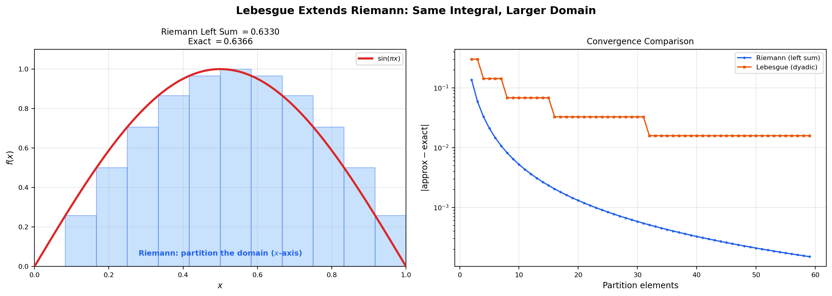
The interactive viz below makes the supremum construction concrete. As you increase the dyadic refinement level, the simple-function staircase climbs upward toward $f$ and the integral climbs upward toward $\int f \, d\mu$ . The supremum is the limit of this climbing process — it is what the construction computes in the limit, not a single staircase you can draw on the page.

Function:levels = 2^3 = 8

∫ s_n dλ = 0.56375Exact ∫ f dλ = 0.63662Error: 7.29e-2

The half-cycle of a sine wave on [0, 1]. Exact integral 2/π ≈ 0.6366. The simple function s_n is the largest dyadic staircase below f at this level — the supremum over all such staircases as n → ∞ is the Lebesgue integral ∫ f dλ.

4. The Integral for General Measurable Functions

So far we have only integrated non-negative functions. To integrate a general measurable function (positive or negative), we split it into its positive and negative parts and integrate each separately.

📐 Definition 3 (Positive and negative parts)

For any measurable function $f: \Omega \to \mathbb{R}$ , define $f^+(x) \;=\; \max(f(x), 0), \qquad f^-(x) \;=\; \max(-f(x), 0).$ Both $f^+$ and $f^-$ are non-negative measurable functions. They satisfy $f \;=\; f^+ - f^-, \qquad |f| \;=\; f^+ + f^-.$

A small visual: $f^+$ keeps the positive parts of $f$ and zeros out the negative parts; $f^-$ does the opposite (and flips the sign so it is also non-negative). Their difference is $f$ , and their sum is $|f|$ . Both are non-negative, so the previous section applies to each.

📐 Definition 4 (Lebesgue integral of a general measurable function)

Let $f: \Omega \to \mathbb{R}$ be a measurable function on $(\Omega, \mathcal{F}, \mu)$ . If at least one of $\int f^+ \, d\mu$ and $\int f^- \, d\mu$ is finite, the Lebesgue integral of $f$ with respect to $\mu$ is $\int f \, d\mu \;=\; \int f^+ \, d\mu \;-\; \int f^- \, d\mu.$ If both are finite, $f$ is Lebesgue-integrable and we write $f \in L^1(\mu)$ . The space $L^1(\mu)$ consists of all measurable functions $f$ with $\int |f| \, d\mu < \infty$ .

The reason we require at least one to be finite is to avoid the indeterminate form $\infty - \infty$ . If both $\int f^+$ and $\int f^-$ are infinite, the integral $\int f$ is left undefined. (In some treatments such functions are called “non-integrable” or “improperly integrable”; we will not need that distinction in this topic.)

📝 Example 6 ($\int_{-\pi}^{\pi} \sin(x) \, d\lambda = 0$ — positive and negative parts cancel)

The function $\sin(x)$ on $[-\pi, \pi]$ is non-negative on $[0, \pi]$ and non-positive on $[-\pi, 0]$ . Its positive part is $\sin^+(x) = \sin(x) \cdot \mathbf{1}_{[0, \pi]}(x)$ and its negative part is $\sin^-(x) = -\sin(x) \cdot \mathbf{1}_{[-\pi, 0]}(x) = \sin(-x) \cdot \mathbf{1}_{[-\pi, 0]}(x)$ . By symmetry, $\int \sin^+ \, d\lambda \;=\; \int_0^{\pi} \sin(x) \, d\lambda \;=\; 2,$ $\int \sin^- \, d\lambda \;=\; \int_{-\pi}^0 -\sin(x) \, d\lambda \;=\; \int_0^{\pi} \sin(x) \, d\lambda \;=\; 2.$ Both integrals are finite, so $\sin \in L^1([-\pi, \pi], \lambda)$ , and $\int \sin \, d\lambda \;=\; 2 - 2 \;=\; 0.$

The definition extends linearity from simple functions to all of $L^1$ , but the proof requires a small bit of bookkeeping.

🔷 Theorem 2 (Linearity of the Lebesgue integral on $L^1(\mu)$)

Let $f, g \in L^1(\mu)$ and $\alpha, \beta \in \mathbb{R}$ . Then $\alpha f + \beta g \in L^1(\mu)$ and $\int (\alpha f + \beta g) \, d\mu \;=\; \alpha \int f \, d\mu + \beta \int g \, d\mu.$

Proof.

The strategy is to reduce to the non-negative case, where linearity is already established (as a limit of the simple-function linearity from Theorem 1).

Step 1: Non-negative linearity. First we extend Theorem 1 from simple functions to general non-negative measurable functions. If $f, g \geq 0$ are measurable and $\alpha, \beta \geq 0$ , choose increasing sequences of non-negative simple functions $s_n \uparrow f$ and $t_n \uparrow g$ (Topic 25, Theorem 5). Then $\alpha s_n + \beta t_n$ is a non-negative simple function with $\alpha s_n + \beta t_n \uparrow \alpha f + \beta g$ . By the definition of the integral as a supremum and Theorem 1 applied at each step, $\int (\alpha f + \beta g) \, d\mu \;=\; \sup_n \int (\alpha s_n + \beta t_n) \, d\mu \;=\; \sup_n \left( \alpha \int s_n + \beta \int t_n \right).$

The sup of a sum of non-negative terms equals the sum of sups (each term is non-decreasing in $n$ ), so this becomes $\alpha \sup_n \int s_n \, d\mu + \beta \sup_n \int t_n \, d\mu \;=\; \alpha \int f \, d\mu + \beta \int g \, d\mu.$

We will give a tighter version of this “sup of sum” step inside the proof of the Monotone Convergence Theorem in Section 5; for now we treat it as the natural extension of Theorem 1 to limits.

Step 2: Subtraction by splitting. For general $f \in L^1(\mu)$ , write $f = f^+ - f^-$ with both $f^+, f^- \in L^1(\mu)$ (their integrals are both finite, since $\int |f| < \infty$ ). Similarly $g = g^+ - g^-$ . The sum $f + g$ has positive and negative parts that satisfy $(f + g)^+ - (f + g)^- \;=\; f + g \;=\; (f^+ + g^+) - (f^- + g^-).$

This identity is the key. The two decompositions of $f + g$ — its own canonical $(f+g)^+ - (f+g)^-$ split, and the sum-of-splits $(f^+ + g^+) - (f^- + g^-)$ — are not the same simple-function decomposition (the second one is “wasteful” in that it can have $f^+$ and $g^-$ both non-zero at the same point, which the canonical decomposition would simplify), but they sum to the same thing. Rearranging: $(f + g)^+ + f^- + g^- \;=\; (f + g)^- + f^+ + g^+.$

Both sides are non-negative measurable functions, so we can apply Step 1 (non-negative linearity) to each. Integrating: $\int (f + g)^+ \, d\mu + \int f^- \, d\mu + \int g^- \, d\mu \;=\; \int (f + g)^- \, d\mu + \int f^+ \, d\mu + \int g^+ \, d\mu.$

All six integrals are finite (everything is in $L^1$ ), so we can rearrange: $\int (f + g)^+ \, d\mu - \int (f + g)^- \, d\mu \;=\; \left[ \int f^+ \, d\mu - \int f^- \, d\mu \right] + \left[ \int g^+ \, d\mu - \int g^- \, d\mu \right].$

The left side is $\int (f + g) \, d\mu$ by Definition 4; the right side is $\int f \, d\mu + \int g \, d\mu$ . So $\int (f + g) \, d\mu = \int f \, d\mu + \int g \, d\mu$ .

Step 3: Scalar multiplication. For $\alpha \geq 0$ , $(\alpha f)^+ = \alpha f^+$ and $(\alpha f)^- = \alpha f^-$ , so $\int \alpha f \, d\mu = \alpha \int f^+ \, d\mu - \alpha \int f^- \, d\mu = \alpha \int f \, d\mu$ . For $\alpha < 0$ , $(\alpha f)^+ = (-\alpha) f^- = |\alpha| f^-$ and $(\alpha f)^- = |\alpha| f^+$ , so $\int \alpha f \, d\mu = |\alpha| \int f^- \, d\mu - |\alpha| \int f^+ \, d\mu = -|\alpha| \int f \, d\mu = \alpha \int f \, d\mu$ . Either way, scalar multiplication pulls through.

Combining additivity (Step 2) and scalar multiplication (Step 3), $\int (\alpha f + \beta g) \, d\mu = \alpha \int f \, d\mu + \beta \int g \, d\mu$ .

∎

💡 Remark 4 (The Lebesgue integral strictly extends the Riemann integral)

If $f: [a, b] \to \mathbb{R}$ is bounded and Riemann-integrable, then $f$ is Lebesgue-integrable on $[a, b]$ (with respect to Lebesgue measure restricted to $[a, b]$ ) and the two integrals agree: $\int_a^b f(x) \, dx \;=\; \int_{[a, b]} f \, d\lambda.$ We will prove this in Section 8 (Theorem 6). The converse is false: the Dirichlet function $\mathbf{1}_{\mathbb{Q}}$ on $[0, 1]$ is Lebesgue-integrable (Example 2) with integral $0$ , but it is not Riemann-integrable (Topic 25, Section 1). So the Lebesgue integral is a strict extension — the same functions as before plus genuinely more.

5. The Monotone Convergence Theorem

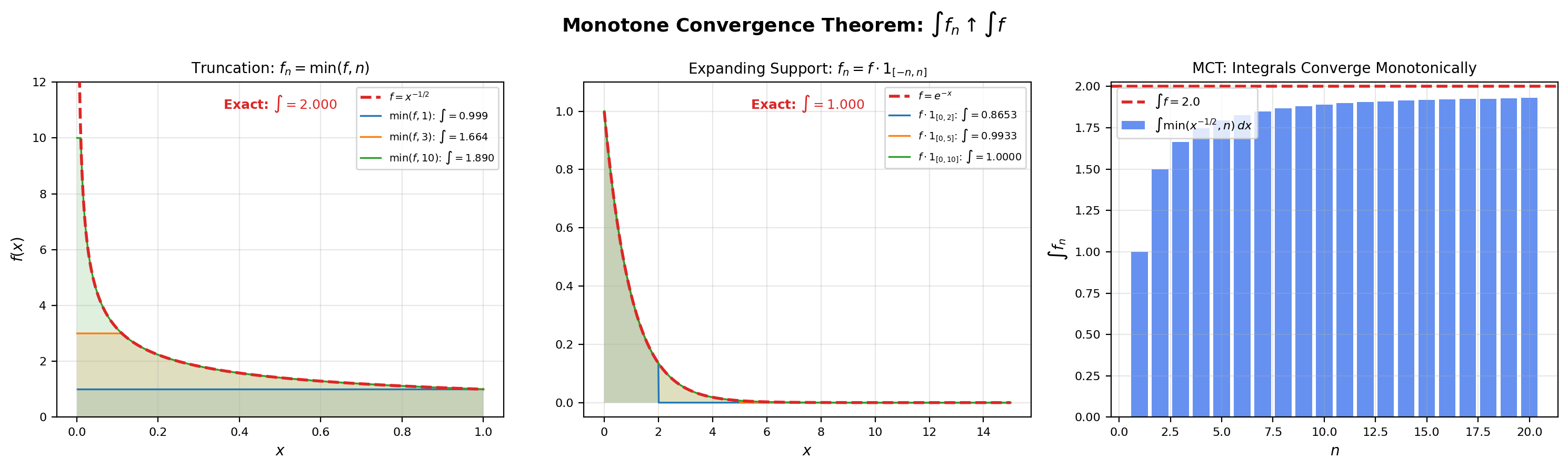
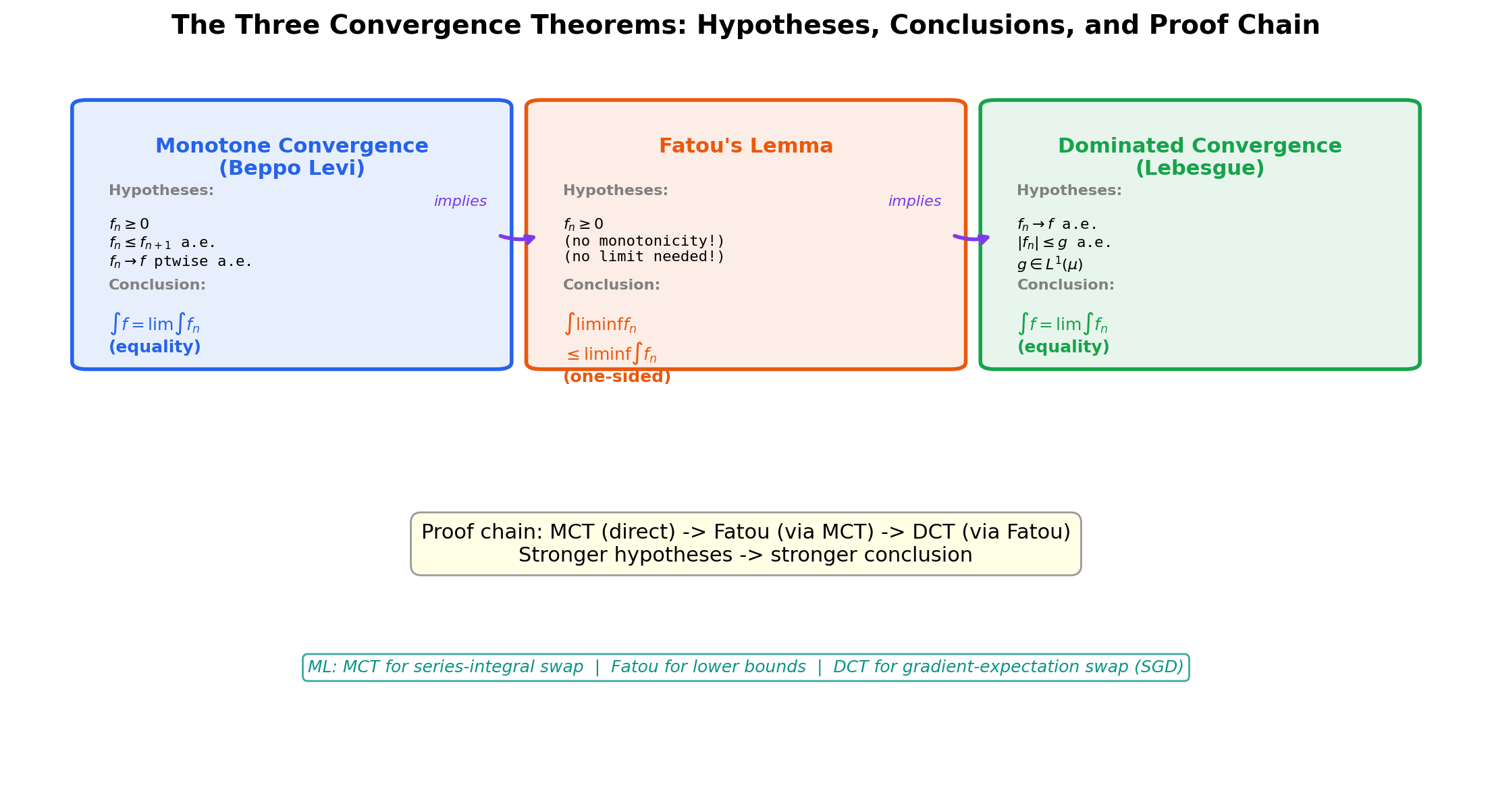
The first of the three convergence theorems. The Monotone Convergence Theorem — historically due to Beppo Levi (1906) — handles the easy case where $(f_n)$ is an increasing sequence. Increasing means we never lose mass, so the limit-integral interchange goes through with no extra hypotheses.

🔷 Theorem 3 (Monotone Convergence Theorem (Beppo Levi))

Let $(f_n)_{n \geq 1}$ be a sequence of non-negative measurable functions on $(\Omega, \mathcal{F}, \mu)$ with $0 \;\leq\; f_1(x) \;\leq\; f_2(x) \;\leq\; \cdots \quad \text{for $\mu$-a.e. } x,$ and let $f(x) = \lim_{n \to \infty} f_n(x)$ be the pointwise limit (which exists in $[0, \infty]$ because the sequence is non-decreasing). Then $f$ is measurable and $\int f \, d\mu \;=\; \lim_{n \to \infty} \int f_n \, d\mu.$

The interactive viz below shows three monotone-convergence sequence types — truncation $f_n = \min(f, n)$ , expanding support $f_n = f \cdot \mathbf{1}_{[-n, n]}$ , and the dyadic simple-function staircase — and the corresponding integral values climbing toward the limit. Try each and see how the bar chart of $\int f_1, \int f_2, \ldots$ converges to $\int f$ from below.

Sequence:n = 5

∫ f_n dμ = 1.80000∫ f dμ = 2.00000Gap (∫ f − ∫ f_n) = 0.20000

Truncate f(x) = 1/√x at height n. As n → ∞ the cap rises and f_n ↑ f. The integrals climb from a small value toward 2 = ∫ f. MCT predicts: ∫ f_n ↑ ∫ f because f_n is non-decreasing and converges pointwise to f.

The proof is the most technically demanding piece of this topic and is worth working through carefully. It is also the prototype for every other “limit and integral commute” argument we’ll see.

Proof.

We must show $\int f \, d\mu = \lim_n \int f_n \, d\mu$ . The plan is to prove $\leq$ and $\geq$ separately. The $\geq$ direction is trivial; the $\leq$ direction is where the work happens.

Step 1: $\lim_n \int f_n \, d\mu \leq \int f \, d\mu$ .

Since $f_n \leq f$ for every $n$ , monotonicity of the integral gives $\int f_n \, d\mu \leq \int f \, d\mu$ for every $n$ . Taking the supremum (which equals the limit because the sequence $\int f_n$ is non-decreasing — a consequence of monotonicity applied to $f_n \leq f_{n+1}$ ), $\lim_{n \to \infty} \int f_n \, d\mu \;=\; \sup_n \int f_n \, d\mu \;\leq\; \int f \, d\mu.$

Step 2: $\int f \, d\mu \leq \lim_n \int f_n \, d\mu$ .

This is the harder direction. By Definition 2, $\int f \, d\mu$ is a supremum over simple functions $s$ with $0 \leq s \leq f$ . So it is enough to show that for every such $s$ , $\int s \, d\mu \;\leq\; \lim_n \int f_n \, d\mu.$

Fix one such simple function $s = \sum_{k=1}^m c_k \mathbf{1}_{A_k}$ with $0 \leq s \leq f$ .

Step 2a: A scaled cutoff trick. Pick any $\alpha \in (0, 1)$ . Define $E_n \;=\; \{x : f_n(x) \geq \alpha \cdot s(x)\}.$

The set $E_n$ is measurable (it is a level set of the difference $f_n - \alpha s$ , which is measurable). Crucially, the sets $E_n$ are increasing: $f_n \leq f_{n+1}$ implies that if $f_n \geq \alpha s$ then $f_{n+1} \geq \alpha s$ , so $E_n \subseteq E_{n+1}$ . And their union covers all of $\Omega$ (well, all of $\Omega$ except a null set): for any fixed $x$ , the sequence $f_n(x)$ converges to $f(x) \geq s(x) > \alpha s(x)$ (the strict inequality holds wherever $s(x) > 0$ because $\alpha < 1$ ; on $\{s = 0\}$ the inequality $f_n \geq 0 = \alpha s$ holds trivially, so $x \in E_n$ for every $n$ ). So $\bigcup_n E_n = \Omega$ up to a null set.

Step 2b: Bound $\int f_n$ from below using $E_n$ . Restrict the integral to $E_n$ : $\int f_n \, d\mu \;\geq\; \int_{E_n} f_n \, d\mu \;=\; \int f_n \cdot \mathbf{1}_{E_n} \, d\mu.$

(The first inequality is monotonicity: $f_n \geq f_n \cdot \mathbf{1}_{E_n}$ pointwise, since the indicator is at most $1$ and $f_n \geq 0$ .) On $E_n$ we have $f_n \geq \alpha s$ by definition, so $\int f_n \cdot \mathbf{1}_{E_n} \, d\mu \;\geq\; \int \alpha s \cdot \mathbf{1}_{E_n} \, d\mu \;=\; \alpha \int s \cdot \mathbf{1}_{E_n} \, d\mu \;=\; \alpha \int_{E_n} s \, d\mu.$

(The second equality uses linearity from Theorem 1.) Combining the two displayed inequalities: $\int f_n \, d\mu \;\geq\; \alpha \int_{E_n} s \, d\mu \;=\; \alpha \sum_{k=1}^m c_k \, \mu(A_k \cap E_n).$

Step 2c: Send $n \to \infty$ . The sets $A_k \cap E_n$ are increasing in $n$ for each $k$ , with union $A_k \cap \bigcup_n E_n = A_k$ (up to a null set). By continuity of measure from below (Topic 25, Theorem 1, second form), $\mu(A_k \cap E_n) \;\xrightarrow[n \to \infty]{}\; \mu(A_k).$

So $\sum_{k=1}^m c_k \, \mu(A_k \cap E_n) \to \sum_{k=1}^m c_k \, \mu(A_k) = \int s \, d\mu$ as $n \to \infty$ . Plugging this into the bound from Step 2b: $\lim_{n \to \infty} \int f_n \, d\mu \;\geq\; \alpha \cdot \int s \, d\mu.$

Step 2d: Send $\alpha \to 1^-$ . The bound $\lim_n \int f_n \, d\mu \geq \alpha \int s \, d\mu$ holds for every $\alpha \in (0, 1)$ . Letting $\alpha \uparrow 1$ , $\lim_{n \to \infty} \int f_n \, d\mu \;\geq\; \int s \, d\mu.$

Step 2e: Take the supremum over $s$ . This bound holds for every simple function $s$ with $0 \leq s \leq f$ . Taking the supremum over all such $s$ on the right and using Definition 2, $\lim_{n \to \infty} \int f_n \, d\mu \;\geq\; \sup_{0 \leq s \leq f} \int s \, d\mu \;=\; \int f \, d\mu.$

This is the inequality we needed. Combined with Step 1, we get equality: $\int f \, d\mu = \lim_n \int f_n \, d\mu$ .

∎

The “scaled cutoff” trick — picking $\alpha < 1$ to give ourselves room, then sending $\alpha \to 1$ at the end — is a recurring move in measure theory. It is the technical engine behind every “lower-semicontinuity” type argument.

📝 Example 7 (Series as integrals against counting measure)

Let $\mu$ be the counting measure on $\mathbb{N}$ : $\mu(A)$ is the cardinality of $A$ for finite $A$ , and $\infty$ otherwise. A function $f: \mathbb{N} \to [0, \infty)$ is just a sequence $(a_k)_{k \geq 1}$ with $a_k = f(k)$ , and the Lebesgue integral against $\mu$ is the sum $\int f \, d\mu = \sum_{k=1}^{\infty} a_k$ .

Apply MCT to the partial-sum sequence $f_n = \sum_{k=1}^n a_k \mathbf{1}_{\{k\}}$ . Each $f_n$ is a non-negative simple function with $\int f_n \, d\mu = \sum_{k=1}^n a_k$ . The sequence is increasing pointwise (each $f_n$ adds one more non-negative term). The limit is $f = \sum_{k=1}^{\infty} a_k \mathbf{1}_{\{k\}}$ , and $\int f \, d\mu = \sum_{k=1}^{\infty} a_k$ . MCT says $\sum_{k=1}^{\infty} a_k \;=\; \int f \, d\mu \;=\; \lim_{n \to \infty} \int f_n \, d\mu \;=\; \lim_{n \to \infty} \sum_{k=1}^n a_k,$ which is just the definition of an infinite series. MCT specializes to “the series of non-negative terms equals the limit of partial sums” — a fact we already knew, but now justified inside the unified Lebesgue framework.

A clean corollary of MCT is the swap of sum and integral for non-negative functions — a result we will use repeatedly.

🔷 Corollary 1 (Sum–integral swap for non-negative functions)

Let $(f_n)_{n \geq 1}$ be a sequence of non-negative measurable functions on $(\Omega, \mathcal{F}, \mu)$ . Then $\int \sum_{n=1}^{\infty} f_n \, d\mu \;=\; \sum_{n=1}^{\infty} \int f_n \, d\mu.$

Proof: apply MCT to the partial sums $S_N = \sum_{n=1}^N f_n$ . The sequence $(S_N)$ is non-negative and increasing, with pointwise limit $\sum_{n=1}^\infty f_n$ . By Theorem 1 (linearity for finite sums of simple functions, then promoted to non-negative measurable functions in Theorem 2 Step 1), $\int S_N \, d\mu = \sum_{n=1}^N \int f_n \, d\mu$ . MCT gives $\int (\sum f_n) \, d\mu = \lim_N \int S_N \, d\mu = \lim_N \sum_{n=1}^N \int f_n \, d\mu = \sum_{n=1}^\infty \int f_n \, d\mu$ .

Three-panel monotone convergence: truncation min(f, n) at n=1, 3, 10 with shaded integrals climbing toward the limit

6. Fatou’s Lemma

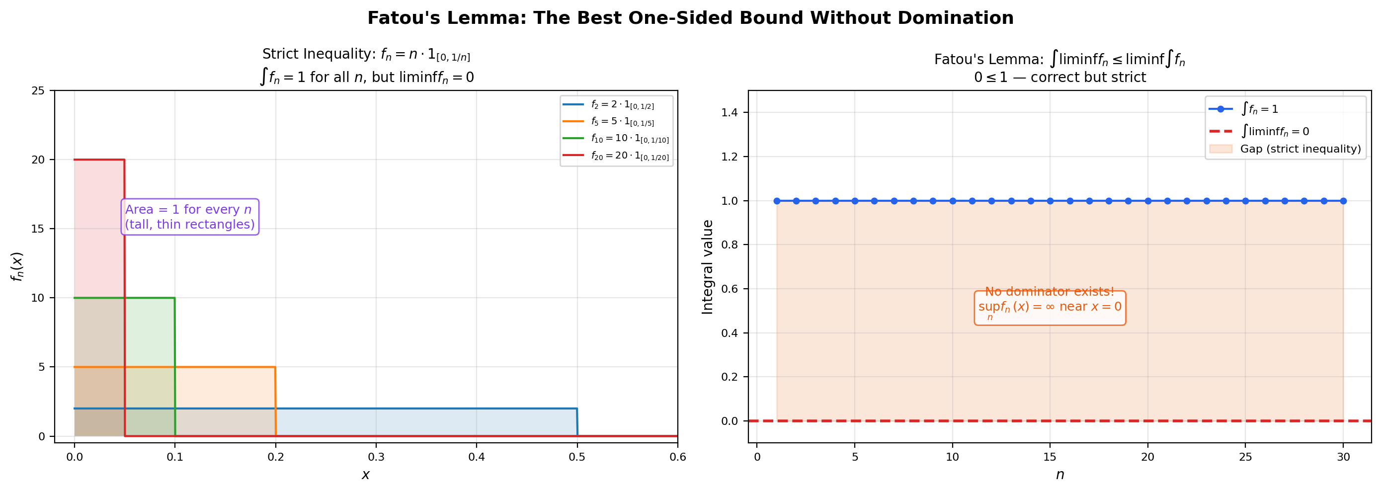
MCT requires the sequence to be increasing. What if it isn’t? Fatou’s Lemma gives the next-best thing: a one-sided inequality that holds for any sequence of non-negative measurable functions, with no monotonicity assumption.

🔷 Theorem 4 (Fatou's Lemma)

Let $(f_n)_{n \geq 1}$ be a sequence of non-negative measurable functions on $(\Omega, \mathcal{F}, \mu)$ . Then $\int \liminf_{n \to \infty} f_n \, d\mu \;\leq\; \liminf_{n \to \infty} \int f_n \, d\mu.$

A reminder on the notation: for any sequence $(a_n)$ of extended reals, $\liminf_n a_n = \lim_{n \to \infty} \inf_{k \geq n} a_k$ — the “eventual” lower bound on the sequence. For functions, $\liminf_n f_n$ is the pointwise $\liminf$ at each point.

Proof.

Define a new sequence $g_n(x) \;=\; \inf_{k \geq n} f_k(x).$

The function $g_n$ is the pointwise infimum of the tail $\{f_n, f_{n+1}, \ldots\}$ . By the standard argument (intersection of measurable level sets), each $g_n$ is measurable and non-negative.

Key observation 1: $(g_n)$ is increasing. As $n$ grows, the set $\{k : k \geq n\}$ shrinks, and the infimum over a smaller set is at least as large as the infimum over a larger set: $g_n \;=\; \inf_{k \geq n} f_k \;\leq\; \inf_{k \geq n + 1} f_k \;=\; g_{n + 1}.$

So $0 \leq g_1 \leq g_2 \leq \cdots$ .

Key observation 2: $g_n \leq f_n$ . Trivially: $g_n$ is the infimum of $\{f_n, f_{n+1}, \ldots\}$ , which includes $f_n$ itself, so $g_n \leq f_n$ pointwise. By monotonicity, $\int g_n \, d\mu \;\leq\; \int f_n \, d\mu.$

Key observation 3: $g_n \to \liminf_n f_n$ . By definition, $\liminf_{n \to \infty} f_n(x) \;=\; \lim_{n \to \infty} \inf_{k \geq n} f_k(x) \;=\; \lim_{n \to \infty} g_n(x).$

So $g_n$ converges pointwise to $\liminf_n f_n$ , and the convergence is monotone-increasing (Observation 1).

Apply MCT to $(g_n)$ . All three hypotheses of MCT hold: $(g_n)$ is non-negative, measurable, and monotone-increasing with pointwise limit $\liminf_n f_n$ . So $\int \liminf_{n \to \infty} f_n \, d\mu \;=\; \int \lim_{n \to \infty} g_n \, d\mu \;=\; \lim_{n \to \infty} \int g_n \, d\mu.$

Combine with Observation 2. From Observation 2, $\int g_n \, d\mu \leq \int f_n \, d\mu$ , so the limit on the left is bounded by the $\liminf$ of the right: $\lim_{n \to \infty} \int g_n \, d\mu \;\leq\; \liminf_{n \to \infty} \int f_n \, d\mu.$

(Note: we use $\liminf$ on the right rather than $\lim$ , because $\int f_n \, d\mu$ does not necessarily converge — it could oscillate. Whatever it does, $\int g_n \to \int \liminf f_n$ from below, and stays below the $\liminf$ of $\int f_n$ .) Combining with the previous display: $\int \liminf_{n \to \infty} f_n \, d\mu \;\leq\; \liminf_{n \to \infty} \int f_n \, d\mu.$

∎

Fatou’s Lemma is a one-sided inequality, and the example below shows that the inequality can be strict — equality is not guaranteed.

📝 Example 8 (Strict inequality in Fatou: the spike sequence)

Take $f_n(x) = n \cdot \mathbf{1}_{[0, 1/n]}(x)$ on $[0, 1]$ — the same sequence from Example 1. Then $f_n(x) \to 0$ pointwise for every $x > 0$ , so $\liminf_n f_n = 0$ everywhere (well, almost everywhere — the value at $x = 0$ tends to $\infty$ , but a single point is null). Therefore $\int \liminf_{n \to \infty} f_n \, d\lambda \;=\; \int 0 \, d\lambda \;=\; 0.$ But $\int f_n \, d\lambda = 1$ for every $n$ , so $\liminf_n \int f_n \, d\lambda = 1$ .

Fatou’s Lemma gives $0 \leq 1$ — correct, but strict. The mass of $f_n$ does not vanish in the integral even though it vanishes pointwise. This is the same phenomenon we observed in Puzzle 1 from Section 1: pointwise convergence does not always imply convergence of integrals.

💡 Remark 5 (Fatou cannot be promoted to equality without extra hypotheses)

The strict inequality in Example 8 shows that Fatou’s Lemma cannot in general be improved to equality. Some additional structure on the sequence $(f_n)$ is required to recover equality. Monotone Convergence gives one such structure (an increasing sequence), and Dominated Convergence in the next section gives another (existence of an integrable dominator). Without one of these extra assumptions, Fatou’s one-sided inequality is the best we can say.

Two-panel Fatou's lemma: strict inequality case with the spike sequence and the integrals staying at 1 while the pointwise limit is 0

7. The Dominated Convergence Theorem

The crown jewel. The Dominated Convergence Theorem is the result that justifies the limit-integral interchange in nearly every modern application — including the gradient–expectation swap that drives stochastic gradient descent.

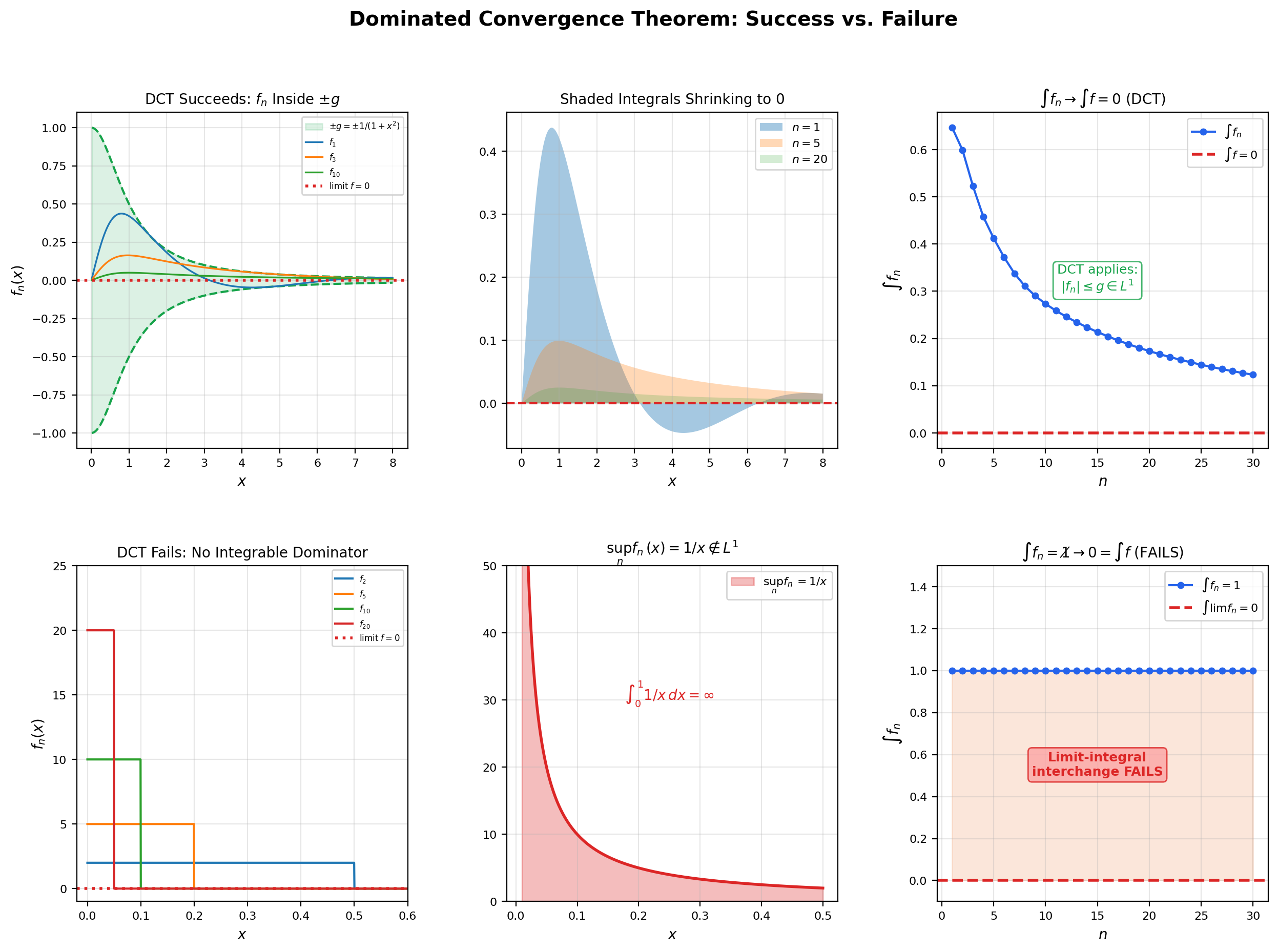
🔷 Theorem 5 (Dominated Convergence Theorem (Lebesgue))

Let $(f_n)_{n \geq 1}$ be a sequence of measurable functions on $(\Omega, \mathcal{F}, \mu)$ with $f_n(x) \to f(x)$ pointwise $\mu$ -a.e. Suppose there exists an integrable function $g \in L^1(\mu)$ (i.e., $\int g \, d\mu < \infty$ ) such that $|f_n(x)| \;\leq\; g(x) \quad \text{for $\mu$-a.e. } x, \text{ for every } n.$ Then $f \in L^1(\mu)$ and $\int f \, d\mu \;=\; \lim_{n \to \infty} \int f_n \, d\mu.$ Equivalently, $\lim_n \int f_n \, d\mu = \int \lim_n f_n \, d\mu$ — limits and integrals commute.

The flagship visualization for this topic is below. It contrasts two scenarios where DCT applies (sequences that have an integrable dominator and whose integrals do converge to the integral of the limit) with one scenario where DCT does not apply (the spike sequence from Example 1, which has no integrable dominator and whose integrals do not converge). Toggle between scenarios and watch the integral history bar chart on the right; the contrast is the conceptual heart of DCT.

Scenario:n = 5Show dominator g

∫ f_n dμ = 0.41990∫ f dμ = 0.00000|∫ f_n − ∫ f| = 0.41990Dominator g is integrable

f_n(x) = sin(x/n) / (1 + x²). As n → ∞ the argument x/n shrinks toward 0, so sin(x/n) → sin(0) = 0 and f_n → 0 pointwise (not by oscillation cancellation, but because the argument itself collapses). Dominator g(x) = 1 / (1 + x²) is integrable on [0, ∞) with ∫ g = π/2, and |sin(x/n)| ≤ 1 gives |f_n| ≤ g. DCT applies, and ∫ f_n → 0 = ∫ f. DCT predicts: ∫ f_n → ∫ f because |f_n| ≤ g and ∫ g < ∞.

The proof uses a slick double-application of Fatou’s Lemma — once to a pair of non-negative sequences manufactured from $f_n$ and the dominator $g$ .

Proof.

The strategy is to apply Fatou’s Lemma to two sequences: $(g + f_n)$ and $(g - f_n)$ . Both are non-negative because $|f_n| \leq g$ implies $-g \leq f_n \leq g$ , so $g + f_n \geq 0$ and $g - f_n \geq 0$ .

Step 1: $f$ is integrable. Pointwise convergence $f_n \to f$ and $|f_n| \leq g$ together imply $|f| \leq g$ . By monotonicity, $\int |f| \, d\mu \;\leq\; \int g \, d\mu \;<\; \infty,$ so $f \in L^1(\mu)$ . The integral $\int f \, d\mu$ is therefore well-defined and finite.

Step 2: Apply Fatou to $g + f_n$ . The sequence $(g + f_n)$ is non-negative and converges pointwise to $g + f$ . Fatou’s Lemma gives $\int (g + f) \, d\mu \;\leq\; \liminf_{n \to \infty} \int (g + f_n) \, d\mu.$

By linearity (Theorem 2), $\int g \, d\mu + \int f \, d\mu \;\leq\; \liminf_{n \to \infty} \left[ \int g \, d\mu + \int f_n \, d\mu \right] \;=\; \int g \, d\mu + \liminf_{n \to \infty} \int f_n \, d\mu.$

(The constant $\int g$ pulls out of the $\liminf$ .) Subtracting $\int g \, d\mu$ from both sides — legal because $\int g \, d\mu$ is finite — we get $\int f \, d\mu \;\leq\; \liminf_{n \to \infty} \int f_n \, d\mu. \tag{$\star$}$

Step 3: Apply Fatou to $g - f_n$ . The sequence $(g - f_n)$ is also non-negative and converges pointwise to $g - f$ . Fatou’s Lemma gives $\int (g - f) \, d\mu \;\leq\; \liminf_{n \to \infty} \int (g - f_n) \, d\mu.$

Linearity again: $\int g \, d\mu - \int f \, d\mu \;\leq\; \int g \, d\mu - \limsup_{n \to \infty} \int f_n \, d\mu.$

The key move on the right: $\liminf_n (-a_n) = -\limsup_n a_n$ , so $\liminf_n (\int g - \int f_n) = \int g - \limsup_n \int f_n$ . Subtract $\int g \, d\mu$ and multiply both sides by $-1$ (which flips the inequality): $\limsup_{n \to \infty} \int f_n \, d\mu \;\leq\; \int f \, d\mu. \tag{$\star\star$}$

Step 4: Combine $(\star)$ and $(\star\star)$ . From $(\star)$ and $(\star\star)$ , $\int f \, d\mu \;\leq\; \liminf_{n \to \infty} \int f_n \, d\mu \;\leq\; \limsup_{n \to \infty} \int f_n \, d\mu \;\leq\; \int f \, d\mu.$

Equality must hold throughout. In particular, $\liminf_n \int f_n = \limsup_n \int f_n$ , which means $\lim_n \int f_n$ exists, and its common value is $\int f \, d\mu$ .

∎

The proof is short once you see the trick: manufacture two non-negative sequences from $f_n$ and the dominator, apply Fatou to each, and let the upper and lower bounds collapse on $\int f$ . The hard work was in MCT (which underlies Fatou); DCT is a clean consequence.

📝 Example 9 (DCT applied: $\int_0^\infty \sin(x/n) / (x^2 + 1) \, dx \to 0$)

For each $n \geq 1$ , define $f_n(x) = \sin(x/n) / (x^2 + 1)$ on $[0, \infty)$ . As $n \to \infty$ , $\sin(x/n) \to \sin(0) = 0$ for every $x$ , so $f_n \to 0$ pointwise. (The convergence is even uniform on bounded intervals.)

We need a dominator. Note that $|\sin(x/n)| \leq 1$ for every $x$ and $n$ , so $|f_n(x)| \;=\; \frac{|\sin(x/n)|}{x^2 + 1} \;\leq\; \frac{1}{x^2 + 1}.$ Set $g(x) = 1 / (x^2 + 1)$ . Then $\int_0^\infty g(x) \, d\lambda = [\arctan(x)]_0^\infty = \pi/2 < \infty$ , so $g$ is integrable. DCT applies, and $\lim_{n \to \infty} \int_0^\infty \frac{\sin(x/n)}{x^2 + 1} \, d\lambda \;=\; \int_0^\infty 0 \, d\lambda \;=\; 0.$ This is the same sequence the flagship viz in this section uses. (Note: the related sequence $f_n(x) = \sin(nx)/(x^2 + 1)$ with high-frequency oscillation also has $\int f_n \to 0$ , but for a different reason — the Riemann-Lebesgue lemma rather than DCT, since $\sin(nx)$ does not converge pointwise. Both reach the same conclusion via different theorems.)

📝 Example 10 (DCT justifies differentiation under the integral sign)

Let $f(x, \theta)$ be a function with the following properties: for each fixed $\theta$ , $f(\cdot, \theta) \in L^1(\mu)$ ; for each fixed $x$ , $f(x, \cdot)$ is differentiable in $\theta$ ; and there is an integrable function $g(x)$ with $\left| \frac{\partial f}{\partial \theta}(x, \theta) \right| \;\leq\; g(x) \quad \text{for $\mu$-a.e. } x, \text{ for every } \theta \in I$ on some interval $I$ containing the point of interest. Then $\frac{d}{d\theta} \int f(x, \theta) \, d\mu(x) \;=\; \int \frac{\partial f}{\partial \theta}(x, \theta) \, d\mu(x).$

The proof is exactly DCT applied to the difference quotient: as $h \to 0$ , the function $\frac{f(x, \theta + h) - f(x, \theta)}{h}$ converges pointwise to $\partial f / \partial \theta$ , and the mean value theorem bounds the difference quotient by $\sup_{\theta' \in I} |\partial f / \partial \theta(x, \theta')| \leq g(x)$ , an integrable dominator. DCT gives the limit-integral swap.

In machine learning, $f(x, \theta) = L(\theta, x)$ is the per-sample loss as a function of parameters and data, and the integral $\int L(\theta, x) \, dP(x) = E_P[L(\theta, X)]$ is the population risk. The displayed identity is exactly the gradient–expectation swap, the move at the heart of every SGD convergence proof: $\nabla_\theta E[L(\theta, X)] = E[\nabla_\theta L(\theta, X)]$ .

💡 Remark 6 (The domination hypothesis is essential — do not skip it)

The spike sequence $f_n = n \cdot \mathbf{1}_{[0, 1/n]}$ from Example 1 is the canonical witness that the domination hypothesis cannot be dropped. Any candidate dominator $g$ would have to satisfy $g \geq n$ on $[0, 1/n]$ for every $n$ , so $g(x) \geq 1/x$ near $x = 0$ , which is not integrable on $(0, 1]$ . There is no integrable dominator. DCT therefore does not apply, and indeed the conclusion fails: $\int f_n = 1$ for every $n$ , but $\int \lim f_n = 0$ . Whenever you write down an SGD-style identity that swaps a limit and an integral, the cost of skipping the domination check is exactly this kind of failure — silent and wrong, with no warning from the theorem.

Three-panel dominated convergence: f_n with dominator envelope, shaded areas, and integral convergence plot

Comparison of the three convergence theorems: hypotheses and conclusions side by side

8. Comparison with the Riemann Integral

Time to tie up Remark 4 from Section 4 with a real proof. Every Riemann-integrable function is Lebesgue-integrable, and the two integrals agree. The Lebesgue integral is therefore a strict extension of the Riemann integral — same answers on the old domain, plus new answers on a larger class of functions.

🔷 Theorem 6 (Riemann-integrable implies Lebesgue-integrable)

Let $f: [a, b] \to \mathbb{R}$ be a bounded function. If $f$ is Riemann-integrable on $[a, b]$ , then $f$ is Lebesgue-integrable on $[a, b]$ (with respect to Lebesgue measure restricted to $[a, b]$ ), and $\int_a^b f(x) \, dx \;=\; \int_{[a, b]} f \, d\lambda.$

Proof.

We give the proof in sketch form; the details are spelled out in Royden §4.3.

The Riemann integral $\int_a^b f(x) \, dx$ exists and equals $V$ if and only if for every $\varepsilon > 0$ there is a partition $P_\varepsilon$ of $[a, b]$ such that $U(f, P_\varepsilon) - L(f, P_\varepsilon) < \varepsilon$ , where $U$ and $L$ are the upper and lower Darboux sums.

The upper and lower Darboux sums are themselves integrals of step functions. Specifically, $L(f, P_\varepsilon) = \int s_\varepsilon \, d\lambda$ where $s_\varepsilon$ is the step function equal to $\inf_{[x_{i-1}, x_i]} f$ on each subinterval, and $U(f, P_\varepsilon) = \int t_\varepsilon \, d\lambda$ where $t_\varepsilon$ takes the supremum on each subinterval. Both $s_\varepsilon$ and $t_\varepsilon$ are simple functions on $[a, b]$ — their integrals exist by Definition 1 and equal the Darboux sums by direct computation.

Refining the partition (taking common refinements as $\varepsilon$ shrinks) produces an increasing sequence of $s_\varepsilon$ ‘s and a decreasing sequence of $t_\varepsilon$ ‘s, with $s_\varepsilon \leq f \leq t_\varepsilon$ everywhere. By Riemann-integrability, $\int t_\varepsilon - \int s_\varepsilon \to 0$ . Taking the pointwise limits $s = \lim s_\varepsilon$ and $t = \lim t_\varepsilon$ (which exist almost everywhere by the increasing/decreasing structure), we get $s \leq f \leq t$ with $\int (t - s) \, d\lambda = 0$ . This forces $s = f = t$ almost everywhere, so $f$ agrees with a measurable function ( $s$ ) almost everywhere, hence $f$ is itself measurable. Applying MCT to $(s_\varepsilon)$ : $\int_{[a, b]} f \, d\lambda \;=\; \int_{[a, b]} s \, d\lambda \;=\; \lim_{\varepsilon \to 0} \int s_\varepsilon \, d\lambda \;=\; \lim_{\varepsilon \to 0} L(f, P_\varepsilon) \;=\; \int_a^b f(x) \, dx.$

The Riemann and Lebesgue values agree.

∎

The converse is much sharper — it tells us exactly which bounded functions are Riemann-integrable. The criterion is purely measure-theoretic: discontinuities only matter on a set of positive measure.

🔷 Theorem 7 (Lebesgue's criterion for Riemann integrability)

Let $f: [a, b] \to \mathbb{R}$ be a bounded function. Then $f$ is Riemann-integrable on $[a, b]$ if and only if the set of points at which $f$ is discontinuous has Lebesgue measure zero.

💡 Remark 7 (Lebesgue's criterion closes the Riemann question)

The “only if” direction is the powerful one: it says Riemann-integrability forces the discontinuity set to be small. Combined with Theorem 6, this gives the complete picture:

The Dirichlet function $\mathbf{1}_{\mathbb{Q}}$ on $[0, 1]$ is discontinuous everywhere (at every point, you can find both rationals and irrationals nearby). The discontinuity set is all of $[0, 1]$ , which has measure $1$ , not $0$ . Lebesgue’s criterion says: not Riemann-integrable. Topic 25’s opening puzzle is now closed at the most precise possible level.
$\mathbf{1}_{\mathbb{Q}}$ is Lebesgue-integrable, with integral $0$ (Example 2). The Lebesgue integral handles it gracefully because it doesn’t care about the discontinuity set as long as the function agrees almost everywhere with a “nice” function (the constant zero, in this case).
A function with finitely many jump discontinuities — a step function, say — has discontinuity set of measure zero, so it is Riemann-integrable. Both integrals agree.

Lebesgue’s criterion is the bridge between the analytic notion of “Riemann-integrable” and the measure-theoretic notion of “almost-everywhere continuous.” It is one of the cleanest results in real analysis: a deep characterization with a one-line statement.

Two-panel Lebesgue vs Riemann: staircase comparison and convergence rates

9. Fubini-Tonelli Theorem

The fourth and final big theorem. Up to this point we have integrated functions of one variable on a single measure space. To integrate functions of two (or more) variables, we need a way to combine measures on different spaces into a product measure on the Cartesian product, and a theorem that lets us compute the resulting integral as an iterated integral (one variable at a time).

This completes the preview from Topic 25, Section 9, where we defined the product sigma-algebra $\mathcal{F}_1 \otimes \mathcal{F}_2$ but stopped short of building the integral on it.

The construction of the product measure $\mu \times \nu$ goes as follows: on rectangles $A \times B$ with $A \in \mathcal{F}_1$ and $B \in \mathcal{F}_2$ , set $(\mu \times \nu)(A \times B) = \mu(A) \cdot \nu(B)$ . Carathéodory’s extension theorem (Topic 25, Theorem 2 in spirit) extends this set function to a $\sigma$ -additive measure on the product sigma-algebra $\mathcal{F}_1 \otimes \mathcal{F}_2$ , provided that both $\mu$ and $\nu$ are $\sigma$ -finite — meaning each space can be written as a countable union of measurable sets of finite measure. (Lebesgue measure on $\mathbb{R}$ is $\sigma$ -finite — write $\mathbb{R} = \bigcup_n [-n, n]$ .) The $\sigma$ -finiteness hypothesis is essential; without it, the product measure construction can fail to be unique.

With $\mu \times \nu$ in hand, we have an integral $\int_{X \times Y} f \, d(\mu \times \nu)$ defined by the same machinery as before. The Fubini-Tonelli theorems tell us that this integral can be computed as an iterated integral.

🔷 Theorem 8 (Tonelli's Theorem)

Let $(X, \mathcal{F}, \mu)$ and $(Y, \mathcal{G}, \nu)$ be $\sigma$ -finite measure spaces, and let $f: X \times Y \to [0, \infty]$ be measurable with respect to the product sigma-algebra $\mathcal{F} \otimes \mathcal{G}$ . Then the maps $x \;\mapsto\; \int_Y f(x, y) \, d\nu(y), \qquad y \;\mapsto\; \int_X f(x, y) \, d\mu(x)$ are measurable on $X$ and $Y$ respectively, and $\int_{X \times Y} f \, d(\mu \times \nu) \;=\; \int_X \left( \int_Y f(x, y) \, d\nu(y) \right) d\mu(x) \;=\; \int_Y \left( \int_X f(x, y) \, d\mu(x) \right) d\nu(y).$

Tonelli is the “non-negative” half of Fubini-Tonelli. Because $f \geq 0$ , all three integrals are non-negative (possibly $+\infty$ ), and the equalities hold without any extra integrability assumption — that is the whole point of Tonelli. For sign-changing functions, we need an additional integrability hypothesis to avoid $\infty - \infty$ ambiguities.

🔷 Theorem 9 (Fubini's Theorem)

Let $(X, \mathcal{F}, \mu)$ and $(Y, \mathcal{G}, \nu)$ be $\sigma$ -finite measure spaces, and let $f: X \times Y \to \mathbb{R}$ be measurable with respect to $\mathcal{F} \otimes \mathcal{G}$ . If $\int_{X \times Y} |f| \, d(\mu \times \nu) \;<\; \infty$ ( $f$ is integrable with respect to the product measure), then $f \in L^1(X \times Y, \mu \times \nu)$ , the iterated integrals exist for $\mu$ -a.e. $x$ (and $\nu$ -a.e. $y$ ), and $\int_{X \times Y} f \, d(\mu \times \nu) \;=\; \int_X \left( \int_Y f(x, y) \, d\nu(y) \right) d\mu(x) \;=\; \int_Y \left( \int_X f(x, y) \, d\mu(x) \right) d\nu(y).$

Proof.

Both theorems are proved by the same four-step “extension by linearity and limits” pattern that runs through all of measure theory.

Step 1: Verify on indicator functions of measurable rectangles. For $f = \mathbf{1}_{A \times B}$ with $A \in \mathcal{F}$ , $B \in \mathcal{G}$ , the iterated integral computation reduces to $\int_X \left( \int_Y \mathbf{1}_{A \times B}(x, y) \, d\nu(y) \right) d\mu(x) \;=\; \int_X \mathbf{1}_A(x) \cdot \nu(B) \, d\mu(x) \;=\; \mu(A) \cdot \nu(B).$ The other iterated order gives the same answer by symmetry, and the product integral is $(\mu \times \nu)(A \times B) = \mu(A) \cdot \nu(B)$ by definition. All three agree.

Step 2: Extend to indicators of measurable sets. A general measurable set $E \in \mathcal{F} \otimes \mathcal{G}$ is built up from rectangles via countable unions, intersections, and complements. The “monotone class theorem” (or equivalently the $\pi$ - $\lambda$ theorem) lets us promote the rectangle case to the general measurable set case. Briefly: the collection of $E$ for which the equality $\int_{X \times Y} \mathbf{1}_E \, d(\mu \times \nu) = \int_X \int_Y \mathbf{1}_E \, d\nu \, d\mu$ holds is closed under increasing unions and complements, and it contains the rectangles, so it contains the entire generated sigma-algebra.

Step 3: Extend to non-negative simple functions, then to non-negative measurable functions. Linearity of the integral promotes Step 2 from indicators to finite linear combinations of indicators (i.e., simple functions). MCT promotes from non-negative simple functions to non-negative measurable functions: choose an increasing sequence of simple functions $s_n \uparrow f$ , apply Step 3 to each $s_n$ , and pass to the limit using MCT on both the inner integral and the outer integral. This gives Tonelli.

Step 4: Extend to general integrable functions. For $f \in L^1(X \times Y, \mu \times \nu)$ , write $f = f^+ - f^-$ . Both $f^+, f^- \geq 0$ and both have finite integrals (since $\int |f| < \infty$ ). Apply Tonelli to each separately and subtract. The integrability hypothesis is what guarantees that the subtraction is unambiguous (no $\infty - \infty$ ). This gives Fubini.

The full details for Steps 2 and 3 occupy several pages and use a careful application of the $\pi$ - $\lambda$ theorem; see Folland §2.5 for the textbook treatment.

∎

The integrability hypothesis in Fubini is essential. Without it, the iterated integrals can disagree even when both exist as improper limits.

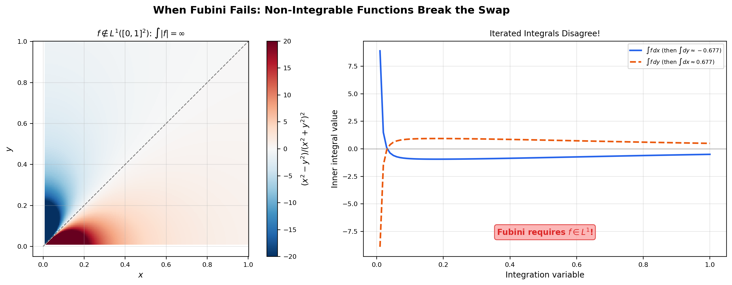
📝 Example 11 (Iterated integrals can disagree without absolute integrability)

Let $f(x, y) = (x^2 - y^2) / (x^2 + y^2)^2$ on $(0, 1] \times (0, 1]$ (extend by $0$ at the origin). A direct computation (or a clever trick: $f = \partial / \partial x [-y / (x^2 + y^2)]$ ) gives $\int_0^1 \int_0^1 \frac{x^2 - y^2}{(x^2 + y^2)^2} \, dy \, dx \;=\; \int_0^1 \left[ \frac{y}{x^2 + y^2} \right]_{y=0}^{y=1} dx \;=\; \int_0^1 \frac{1}{1 + x^2} \, dx \;=\; \frac{\pi}{4},$ $\int_0^1 \int_0^1 \frac{x^2 - y^2}{(x^2 + y^2)^2} \, dx \, dy \;=\; -\frac{\pi}{4} \quad \text{(by the same computation with $x \leftrightarrow y$, picking up a sign).}$

The two iterated integrals exist (as improper Riemann integrals) and disagree. Fubini tells us that this can only happen when the integrability hypothesis fails, and indeed $\int_0^1 \int_0^1 |f(x, y)| \, dy \, dx = \infty$ — the singularity at the origin is bad enough that the function is not absolutely integrable on $(0, 1]^2$ . The product integral $\int f \, d(\lambda \times \lambda)$ does not exist.

📝 Example 12 ($E[XY] = E[X] \cdot E[Y]$ for independent random variables via Fubini)

Let $X, Y$ be independent real-valued random variables on a probability space $(\Omega, \mathcal{F}, P)$ . Independence means the joint distribution of $(X, Y)$ on $\mathbb{R}^2$ is the product measure $P_X \otimes P_Y$ (this is the formal definition of independence — see Topic 25, Remark 10). Suppose $E|X|, E|Y| < \infty$ .

The expected value $E[XY] = \int xy \, d(P_X \otimes P_Y)$ . By Fubini (the integrability hypothesis follows from $|xy| = |x| \cdot |y|$ and Tonelli applied to $|x| \cdot |y|$ , which gives $\int |xy| \, d(P_X \otimes P_Y) = E|X| \cdot E|Y| < \infty$ ), $E[XY] \;=\; \int xy \, d(P_X \otimes P_Y) \;=\; \int_{\mathbb{R}} \left( \int_{\mathbb{R}} xy \, dP_Y(y) \right) dP_X(x) \;=\; \int_{\mathbb{R}} x \cdot E[Y] \, dP_X(x) \;=\; E[X] \cdot E[Y].$

This is the textbook identity “expectation factors over independent variables.” The proof is one application of Fubini. The same argument extends to any finite collection of independent random variables and is the foundation of every “weak law of large numbers” computation.

💡 Remark 8 (Fubini connects back to Topic 13)

The measure-theoretic Fubini theorem (Theorem 9) is the generalization of the Riemann-integral Fubini theorem from Multiple Integrals & Fubini’s Theorem. Same statement — “swap the order of iterated integration” — but now valid on arbitrary $\sigma$ -finite measure spaces, not just $\mathbb{R}^n$ with Lebesgue measure. In particular, Tonelli’s theorem applied to non-negative integrands on $\mathbb{R}^2$ recovers the Topic 13 statement that the order of integration is irrelevant for non-negative continuous functions on a rectangle, and Fubini extends the result to the much broader class of $L^1$ functions on arbitrary product measure spaces (e.g., probability times probability, counting times Lebesgue, $\sigma$ -finite times $\sigma$ -finite). The Topic 13 version was already enough for almost all calculus computations; the Topic 26 version is what probability theory and functional analysis need.

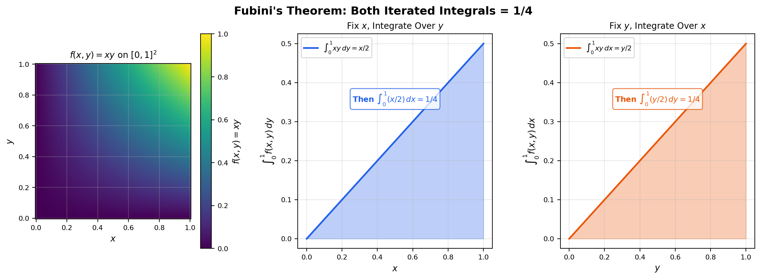
The interactive viz below lets you choose a function on $[0, 1]^2$ and see all three integrals — both iterated orderings and the product integral — computed simultaneously. For the smooth and separable cases, all three agree. For the pathological case from Example 11, the iterated integrals disagree visibly.

Function:

∫₀¹ ∫₀¹ f dy dx = 0.25000∫₀¹ ∫₀¹ f dx dy = 0.25000∫ f d(λ × λ) = 0.25000✓ all three agree

f(x, y) = xy on [0, 1]². Smooth and integrable. All three integrals agree at 1/4.

Three-panel Fubini iterated: heatmap of f(x,y), slice plot, and final integral values

Two-panel Fubini pathological: heatmap of (x²-y²)/(x²+y²)² and the disagreeing iterated integrals

10. Computational Notes

A few practical notes on how the Lebesgue integral surfaces in scientific Python.

Numerical integration as Lebesgue approximation. scipy.integrate.quad computes $\int_a^b f(x) \, dx$ using adaptive Gauss-Kronrod quadrature. Conceptually, this is a sophisticated version of the simple-function supremum from Definition 2: it samples $f$ at strategically chosen points, computes a weighted sum, and refines until the estimated error is below a tolerance. The key practical difference from the theoretical definition is that the computer uses finitely many function evaluations (typically 21–63 in a single call), while the Lebesgue supremum is over all simple functions $\leq f$ . For smooth integrands the convergence is fast enough that the difference is invisible; for integrands with singularities or oscillations, you can hit the tolerance limit and need adaptive subdivision (scipy.integrate.quad does this automatically) or specialized methods.

Monte Carlo integration. For high-dimensional integrals — say $\int_{\mathbb{R}^d} f(x) \, dP(x)$ with $d \geq 5$ — quadrature methods scale exponentially in $d$ and become unusable. The alternative is Monte Carlo: sample $X_1, \ldots, X_N$ independently from $P$ and estimate $\int f \, dP \;\approx\; \frac{1}{N} \sum_{i=1}^N f(X_i).$ The strong law of large numbers (which is itself a corollary of MCT and the first Borel-Cantelli lemma from Topic 25) guarantees almost-sure convergence as $N \to \infty$ . The standard error scales as $\sigma_f / \sqrt{N}$ , where $\sigma_f^2 = \mathrm{Var}_P[f(X)]$ — the dimension does not appear. This is the reason every modern probabilistic ML algorithm (variational inference, MCMC, importance sampling, score matching) is built on Monte Carlo rather than quadrature.

torch.distributions and expected values. Every call to dist.mean, dist.variance, or dist.entropy() is computing a Lebesgue integral against the distribution dist. The .log_prob(x) method returns $\log p(x) = \log (dP / d\lambda)(x)$ — the log of the Radon-Nikodym derivative of the distribution with respect to Lebesgue measure (when one exists). For discrete distributions, the same method returns $\log p(x) = \log P(\{x\})$ — the log probability of the singleton set. The same code path handles both cases because torch.distributions is built on top of a measure-theoretic abstraction in which the underlying reference measure (Lebesgue or counting) is implicit. Topic 28 (Radon-Nikodym) will make this connection precise.

The numerical pitfall: verifying the DCT hypothesis. In practice, finding an integrable dominator $g$ is the hardest part of applying DCT correctly. For a parametric family $f(x, \theta)$ , a common strategy is to dominate by the envelope $\sup_{\theta \in \Theta} |f(x, \theta)|$ over a compact parameter set $\Theta$ , and verify integrability of the envelope numerically. When you can’t find a dominator, you usually have to fall back on a weaker convergence theorem (Vitali convergence, dominated convergence in measure) or do the computation a different way. If your training loop is silently producing biased gradient estimates, it is likely because you implicitly invoked DCT in a place where the dominator does not exist — exactly the failure mode of the spike sequence in Example 1.

📝 Example 13 (Monte Carlo estimation of $E[\sin(X)]$ for $X \sim \mathrm{Exp}(1)$)

Let $X$ be an exponential random variable with rate $1$ , so $X$ has density $p(x) = e^{-x}$ on $[0, \infty)$ . We want $E[\sin(X)] = \int_0^\infty \sin(x) e^{-x} \, dx$ .

A direct integration (integration by parts twice, or recognizing the Laplace transform of $\sin$ ) gives $\int_0^\infty \sin(x) e^{-x} \, dx \;=\; \frac{1}{1 + 1^2} \;=\; \frac{1}{2}.$

Monte Carlo: draw $X_1, \ldots, X_N$ i.i.d. from $\mathrm{Exp}(1)$ and form $\hat{m}_N = (1/N) \sum_i \sin(X_i)$ . By the strong law of large numbers, $\hat{m}_N \to 1/2$ almost surely. The standard error is $\sigma / \sqrt{N}$ where $\sigma^2 = \mathrm{Var}[\sin(X)] = E[\sin^2(X)] - (1/2)^2$ . A short numerical experiment with $N = 10^6$ typically gives $\hat{m}_N$ within $\pm 0.001$ of $0.5$ .

import numpy as np
N = 10**6
X = np.random.exponential(1.0, size=N)
estimate = np.mean(np.sin(X))
print(estimate)  # ≈ 0.5

The convergence rate $1/\sqrt{N}$ is independent of dimension, which is why the same script generalizes — without modification — to estimating $E[g(X_1, \ldots, X_d)]$ for $d = 100$ or $d = 10{,}000$ .

11. Connections to ML

Four big connections, each substantial enough to be its own research thread.

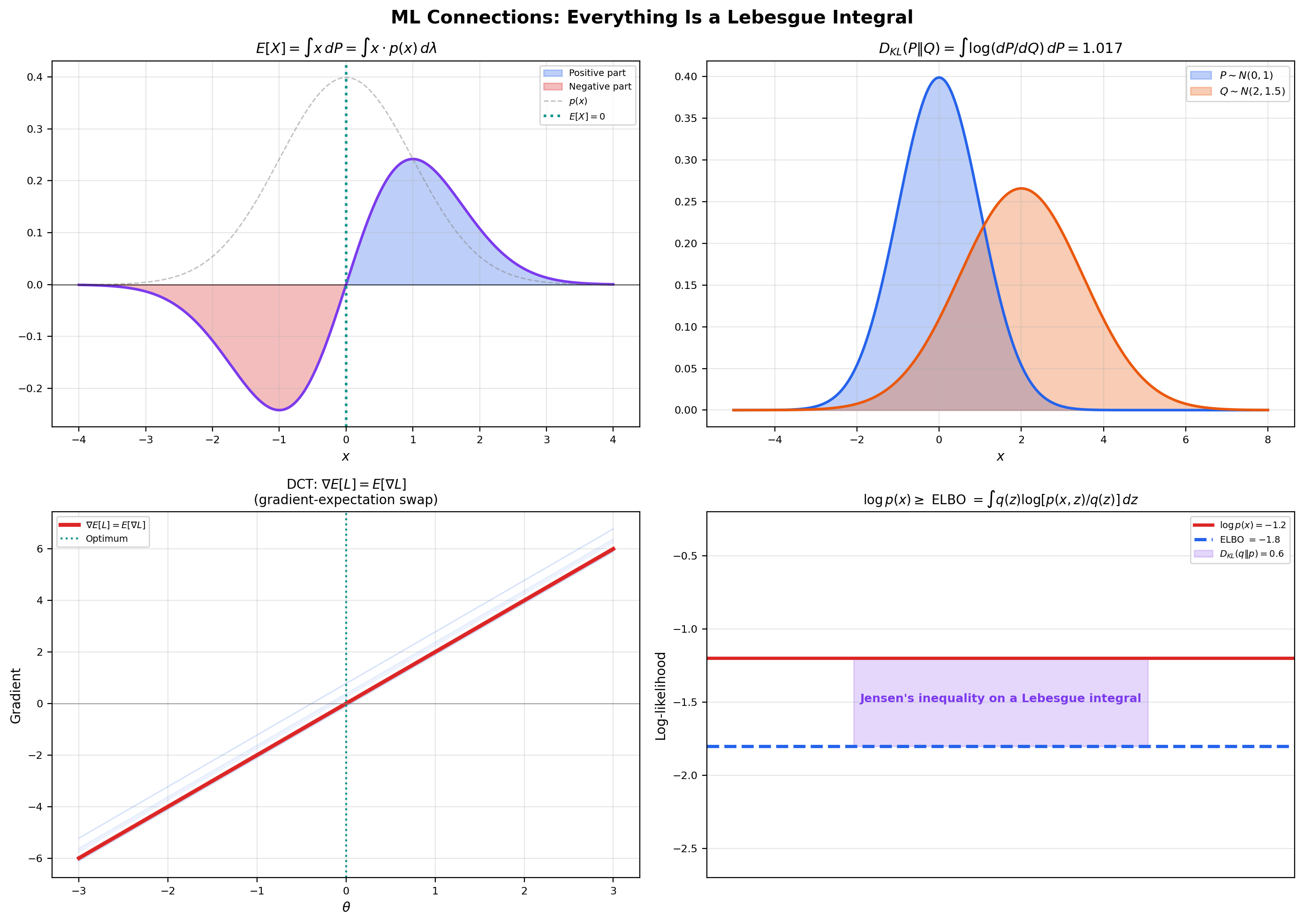
Expected value as a Lebesgue integral. The expected value of a real random variable $X$ on a probability space $(\Omega, \mathcal{F}, P)$ is, by definition, the Lebesgue integral $E[X] \;=\; \int_\Omega X \, dP \;=\; \int_\Omega X(\omega) \, dP(\omega).$

This single definition unifies all the textbook formulas you have seen in elementary probability. For a discrete random variable taking values $x_1, x_2, \ldots$ with probabilities $p_1, p_2, \ldots$ , the integral against $P$ becomes the sum $E[X] = \sum_k x_k p_k$ . For a continuous random variable with density $p(x)$ with respect to Lebesgue measure, the integral becomes $E[X] = \int_{\mathbb{R}} x \cdot p(x) \, dx$ . For the mixture cases that appeared in Puzzle 2 of Section 1, the integral handles the discrete and continuous components in a single uniform formula. Every higher moment ( $E[X^k]$ ), every moment generating function ( $E[e^{tX}]$ ), and every characteristic function ( $E[e^{itX}]$ ) is a Lebesgue integral against $P$ . The Lebesgue integral is what makes “expectation” a single mathematical operation rather than a family of formulas. Forward link: Probability Spaces.

KL divergence and cross-entropy as Lebesgue integrals. The Kullback-Leibler divergence between two probability measures $P, Q$ on a common measurable space, with $P \ll Q$ (meaning $P$ is absolutely continuous with respect to $Q$ ), is $D_{\mathrm{KL}}(P \,\|\, Q) \;=\; \int \log \frac{dP}{dQ} \, dP.$

The integrand $\log (dP/dQ)$ is the log of a Radon-Nikodym derivative — a measurable function on the underlying space. The integral is taken with respect to $P$ . KL divergence is non-negative (a consequence of Jensen’s inequality applied to the convex function $-\log$ , which is itself a Lebesgue integral inequality), zero iff $P = Q$ a.e., and convex in both arguments. None of these properties is provable without the Lebesgue framework; they all use integral inequalities that require absolute integrability and the linearity from Theorem 2.

The cross-entropy $H(P, Q) = -\int \log(dQ / d\lambda) \, dP$ — the loss function for classification when $Q$ is the model’s predictive distribution and $P$ is the empirical distribution of the training labels — is the same kind of object: a Lebesgue integral of a log-density against a probability measure. Forward link: Information Geometry.

SGD as Dominated Convergence. This is the connection from Puzzle 3 of Section 1 and Example 10 of Section 7. The identity $\nabla_\theta E[L(\theta, X)] \;=\; E[\nabla_\theta L(\theta, X)]$ is the mathematical move that makes minibatch gradient descent an unbiased estimator of full-batch gradient descent. The interchange is justified by the Dominated Convergence Theorem applied to the difference quotients in $\theta$ , with the dominator coming from any uniform Lipschitz bound on $\nabla_\theta L$ . In practice, gradient clipping and bounded-support data assumptions are the operational ways to ensure a dominator exists. Every SGD convergence proof in the optimization literature (Robbins-Monro, Nesterov, Adam, anything in the deep learning theory canon) implicitly invokes DCT at this step. Forward link: Gradient Descent.

The ELBO and Jensen’s inequality on integrals. In variational inference, we want to compute the marginal likelihood $\log p(x) = \log \int p(x, z) \, dz$ , which is intractable for most interesting models. The trick is to introduce a tractable variational distribution $q(z)$ and use Jensen’s inequality: $\log p(x) \;=\; \log \int p(x, z) \, dz \;=\; \log \int \frac{p(x, z)}{q(z)} \cdot q(z) \, dz \;=\; \log E_q\left[ \frac{p(x, z)}{q(z)} \right] \;\geq\; E_q\left[ \log \frac{p(x, z)}{q(z)} \right].$

The last step is Jensen’s inequality on the concave function $\log$ , applied to the random variable $p(x, Z) / q(Z)$ under the law $q$ . The right-hand side is the evidence lower bound (ELBO): $\mathrm{ELBO}(q) \;=\; E_q\left[ \log p(x, Z) \right] - E_q\left[ \log q(Z) \right].$

Jensen’s inequality is a Lebesgue integral inequality — it requires $\log$ being concave plus integrability of both sides, both of which are statements about the integral defined in this topic. The tightness of the ELBO (the gap $\log p(x) - \mathrm{ELBO}(q)$ ) is exactly the KL divergence $D_{\mathrm{KL}}(q \,\|\, p(\cdot \mid x))$ , which is itself a Lebesgue integral. The whole machinery of variational inference is integral inequalities all the way down. Forward link: Variational Inference.

📝 Example 14 (KL divergence between two Gaussians as a closed-form Lebesgue integral)

Let $P = \mathcal{N}(\mu_1, \sigma_1^2)$ and $Q = \mathcal{N}(\mu_2, \sigma_2^2)$ be two univariate Gaussians on $\mathbb{R}$ . Both are absolutely continuous with respect to Lebesgue measure, with densities $p_1(x), p_2(x)$ . The Radon-Nikodym derivative $dP/dQ$ at $x$ is $p_1(x) / p_2(x)$ , so $D_{\mathrm{KL}}(P \,\|\, Q) \;=\; \int \log \frac{p_1(x)}{p_2(x)} \cdot p_1(x) \, dx \;=\; E_{X \sim P}\left[ \log \frac{p_1(X)}{p_2(X)} \right].$

Plugging in the Gaussian densities and evaluating the integral (which is a finite computation involving $E_P[X]$ and $E_P[X^2]$ ), the answer is $D_{\mathrm{KL}}(P \,\|\, Q) \;=\; \log \frac{\sigma_2}{\sigma_1} + \frac{\sigma_1^2 + (\mu_1 - \mu_2)^2}{2 \sigma_2^2} - \frac{1}{2}.$

This closed form is used inside the reparametrization-trick KL term of the variational autoencoder loss — every VAE that assumes Gaussian posterior and Gaussian prior ships this expression in its loss function.

📝 Example 15 (Verifying the DCT hypothesis for $L^2$-regularized SGD)

Suppose the per-sample loss is $L(\theta, x) = \ell(\theta, x) + (\lambda / 2) \|\theta\|^2$ for some baseline loss $\ell$ and regularization strength $\lambda > 0$ . The gradient is $\nabla_\theta L(\theta, x) = \nabla_\theta \ell(\theta, x) + \lambda \theta$ .

Suppose $\nabla_\theta \ell$ is uniformly bounded: $|\nabla_\theta \ell(\theta, x)| \leq G$ for all $\theta$ in a compact set $\Theta$ and $\mu$ -a.e. $x$ . (This is the standard “bounded gradient” assumption that holds for any logistic-regression-style model with bounded features.) Then for $\theta \in \Theta$ , $|\nabla_\theta L(\theta, x)| \;\leq\; G + \lambda \cdot \mathrm{diam}(\Theta) \;:=\; M.$

The constant $M$ is finite. The constant function $g(x) = M$ is integrable with respect to any probability measure $P$ on $\mathbb{R}^d$ (its integral is just $M$ ). So the DCT hypothesis is satisfied with dominator $g \equiv M$ , and the interchange $\nabla_\theta E[L(\theta, X)] = E[\nabla_\theta L(\theta, X)]$ is justified for $\theta \in \Theta$ . The minibatch gradient is therefore an unbiased estimator of the population gradient — this is the precise statement that makes SGD work, and the verification took three lines once we knew the dominator structure to look for.

Four-panel ML connections: expected value, KL divergence, gradient-expectation swap, and the ELBO

12. Connections & Further Reading

This is the second topic in Track 7 — Measure & Integration — and the second advanced topic in formalCalculus. Topic 25 built the framework; this topic built the integral. The combination is what makes measure theory a usable tool, not just a piece of mathematical infrastructure: every theorem in this topic is the rigorous version of an everyday calculation in probability theory or machine learning. The next two topics in the track will build the function spaces ( $L^p$ ) and the change-of-measure machinery (Radon-Nikodym) that complete the foundation for modern probability.

If the convergence-theorem proofs felt harder than the proofs in Topic 25, that is accurate, and it is the natural difficulty step-up of moving from “set-theoretic reasoning about measures” to “limit-of-integrals manipulations.” The MCT proof technique (the scaled cutoff $\alpha < 1$ , the increasing exhaustion $E_n \uparrow \Omega$ , the diagonal sup over simple functions) is the prototype for almost every proof in measure-theoretic real analysis from this point forward.

Within formalCalculus:

Sigma-Algebras & Measures — Every concept used here was built in Topic 25: sigma-algebras, measures, measurable functions, simple functions, null sets, “almost everywhere,” product sigma-algebras, and the simple-function approximation theorem. Topic 26 is a direct continuation of Topic 25; if any of those tools is unfamiliar, Topic 25 is the place to refresh.
The Riemann Integral & FTC — Section 8 proves that every Riemann-integrable function is Lebesgue-integrable with the same value. Lebesgue’s criterion (Theorem 7) is the cleanest possible characterization of Riemann-integrability, and it is a measure-theoretic statement: the discontinuity set must have measure zero.
Multiple Integrals & Fubini’s Theorem — Section 9’s measure-theoretic Fubini-Tonelli generalizes the Riemann-integral version from Topic 13. Same statement, broader domain.

Successor topic now published:

$L^p$ Spaces — Banach spaces of measurable functions where $\|f\|_p = (\int |f|^p \, d\mu)^{1/p} < \infty$ . Equivalence classes under a.e.-equality. The completeness theorem (Riesz-Fischer) is a direct application of the Dominated Convergence Theorem from Section 7 — the $L^p$ norm is exactly the right tool to make the convergence-theorem machinery into a complete metric space structure on functions.

Successor topics within formalCalculus:

Radon-Nikodym & Probability Densities — Characterizes when one measure $\nu$ has a density $f = d\nu/d\mu$ with respect to another measure $\mu$ . The bridge from measure theory to probability densities, conditional expectation, and Bayesian inference. The KL-divergence and importance-sampling formulas from Section 11 of this topic are special cases that we formalize there.

Forward to formalml.com:

Probability Spaces — Expected value $E[X] = \int X \, dP$ is the central operation in probability theory, and it is exactly the Lebesgue integral built in this topic. Every moment, MGF, characteristic function, and conditional expectation in probability theory is an instance of this integral.
Gradient Descent — The interchange $\nabla_\theta E[L(\theta, X)] = E[\nabla_\theta L(\theta, X)]$ is the single most-cited DCT application in machine learning. Every SGD convergence proof in the optimization literature implicitly invokes the Dominated Convergence Theorem from Section 7 of this topic.
Information Geometry — KL divergence $D_{\mathrm{KL}}(P \,\|\, Q) = \int \log(dP/dQ) \, dP$ and cross-entropy are Lebesgue integrals against probability measures. Their analytic properties (non-negativity via Jensen, convexity, lower semicontinuity) are integral inequalities provable inside the framework of this topic.
Variational Inference — The evidence lower bound is Jensen’s inequality applied to a Lebesgue integral. The tightness gap is a KL divergence, which is itself a Lebesgue integral. The entire variational machinery is integral inequalities on Lebesgue integrals.

References:

Royden, H. L. & Fitzpatrick, P. M. Real Analysis (4th ed., 2010), Chapters 4 and 18. The closest match to our exposition order — Chapter 4 covers Lebesgue integration on $\mathbb{R}$ with the same supremum-of-simple-functions construction we used in Section 3, and Chapter 18 generalizes to abstract measure spaces.
Folland, G. B. Real Analysis: Modern Techniques and Their Applications (2nd ed., 1999), Chapters 2 and 3. The reference for the Tonelli/Fubini proof sketch in Section 9. Concise, rigorous, graduate-level.
Tao, T. An Introduction to Measure Theory, Chapters 1.4–1.6. Free PDF, written with the same geometric-first instinct that drives this curriculum.
Billingsley, P. Probability and Measure (3rd ed., 1995), Chapters 3–4. The probability-flavored treatment, closest to our ML-connection sections.

References

book Royden, H. L. & Fitzpatrick, P. M. (2010). Real Analysis Fourth edition. Chapters 4 (Lebesgue integration on ℝ) and 18 (general measure spaces). Closest to our exposition order.
book Folland, G. B. (1999). Real Analysis: Modern Techniques and Their Applications Second edition. Chapter 2 (integration), Chapter 3 (signed measures). Concise and rigorous; the source for our Tonelli/Fubini proof sketch.
book Tao, T. (2011). An Introduction to Measure Theory Free PDF. Chapters 1.4–1.6 (the integral on ℝ, then abstract). Pedagogically closest to our geometric-first approach.
book Billingsley, P. (1995). Probability and Measure Third edition. Chapters 3–4 (integration, expected values). Probability-flavored treatment closest to our ML connections.